Lecture 15
Analysis of Policy Interventions

Esteban Moro

Network Science Institute | Northeastern University

NETS 7983 Computational Urban Science

2025-04-15

Welcome!

This week:

Analysis of Policy Interventions in Computational Urban Science

You are here

Data -> Methods -> Models -> Applications.

Aims

• Understand policy evaluation and how it is often done
• How we can use computational tools (causal inference) and large-scale datasets to improve policy evaluation
• Showcase some recent examples of the use of CUS in policy evaluation

Contents

• Policy evaluation
• Use of CUS in policy evaluation
• Examples:
  • Effects of congestion pricing in NYC
  • Measuring the impact of slow zones on street life using social media
  • Effects of EV charging stations on business
• Conclusions
• Further reading
• References

Policy evaluation

Policy evaluation

Cities are the largest laboratories of policy innovation: transport, housing, climate, equity.

Policies need to be:

• Efficiently designed
• Correctly deployed
• Properly evaluated

The critical part is “Evaluation”, i.e., knowing what is the effect of the policy in different groups/areas/times so we can re-design or calibrate our policy for a more efficient implementation.

Thus, we need an accurate policy evaluation framework based on data collection, causal inference, and prediction models.

Policy evaluation

Ideally, that policy evaluation framework should be a Randomized Control Trial. However, ethical, economic, justice, or legal restrictions prevent that possibility. Most of the times we have only observational data about the impact of policies.

This comes with key challenges:

• Selection bias: treated groups/areas are not selected randomly in the city
• Spillover effects: sometimes policies end up affecting groups/areas not considered initially
• Complex, dynamic systems: specific policies might ripple across other systems/areas/group

Policy evaluation

Because of their complexity, policy evaluation is typically done using very simple techniques:

• Simple correlation: “less cars, more business activity”
  • Just runs correlations or regressions between treatment and outcome
  • Ignores reverse causality, omitted variables
  • Confuses association with causation.
• Before-after comparison: “we built the bike lane… and cycling increased”. This kind of comparisons
  • Ignores seasonality, long-term trends
  • Fails to establish a counterfactual.

Policy evaluation

Because of their complexity, policy evaluation is typically done using very simple techniques:

• Treated-only analysis: “areas with new EV chargers saw more food traffic than the city average”.
  • Compares treated units to citywide or unmatched averages
  • Ignores baseline differences between areas
  • Confounds policy effects with selection bias.
• Simple geographical analysis “we compare areas with new EV charges with those around them”
  • Ignores potential spill-over effects and SUTVA
  • Overestimate/Underestimate effects
  • Misses potential negative externalities.

Policy evaluation

For those reasons, typical policy evaluation

• Overestimates the effect of the intervention, because of selection bias, externalities, confounders, etc.

• Does not scale, because evaluations focus only on the direct, local impact without considering systemic feedbacks or spillovers.

• Misses unintended consequences, such as gentrification, traffic rerouting, or increased inequities — especially when only immediate or positive effects are measured.

• Fails to capture dynamic and spatial effects, assuming impact is contained and static. Example: Retail policies in one neighborhood may shift customer flows rather than grow them.

• Leads to misleading narratives, reinforcing decisions based on anecdotal evidence or correlation rather than robust evidence.

Policy evaluation

Example: using before-after comparisons to evaluate the impact of transportation policies:

Use of CUS in policy evaluation

The use of large-scale data and computational tools allows for more accurate, scalable, and nuanced policy evaluation by:

• More statistical power: As we said, most policies result in small changes in behavior. Also, we can break down the effect of intervention by, e.g., demographic group.
• Capturing city-wide dynamics: Instead of isolated pilot areas, CUS tools can track interventions affecting the entire urban area
• Building better counterfactuals: Through causal inference methods (e.g., DiD, matching, synthetic control), CUS can simulate what would have happened in the absence of the policy.
• Using real-time behavioral data: High-resolution data from mobile phones, sensors, or platforms lets us measure actual behavior change — not just intentions or assumptions.
• Enabling iterative evaluation: Continuous data streams allow for monitoring and adjusting policies in near real-time.

Use of CUS in policy evaluation

Key challenges in using CUS or policy evaluation:

• Causal identification is hard: it requires careful design of the quasi-experimental setting
• Spillovers: Policies often affect areas beyond their immediate target.
• Defining treatment and exposure: Proximity doesn’t always equal exposure or impact.
• Data heterogeneity, bias and noise: large-scale data offers quantity and coverage, but comes with bias, quality, interpretation, and noise problems.
• Ethical and privacy concerns: Using behavioral and location data raises important questions about consent, representation, and algorithmic bias.

Use of CUS in policy evaluation

Roadmap:

• Data: check the representativity of the data. Areas, people, temporal coverage. Try to

• Quasi-experimental design:

  • Define the treated and control group controlling for selection bias or potential spill-overs
  • Use propensity score matching or other techniques to balance the groups
  • Use large-scale data to identify potential spill-overs

• Estimation of the impact:

  • Control for potential confounders.
  • Use synthetic control to control for parallel trends.
  • Use DiD when you cannot fully find the set of confounders.

Use of CUS in policy evaluation

• Statistical analysis of the impact:
  • Check the robustness of your impact to basic assumptions made above.
  • Run a placebo test to see if your results are still due to hidden correlations.
• Compare:
  • Most policies happen in different places at the same time.
  • If possible, use other datasets to assess the impact of our source of behavioral data. Use also surveys to understand people’s thinking

Examples

Example: effects of congestion pricing in NYC

NYC launched a congestion pricing program aimed at reducing traffic congestion in Manhattan below 60th St.

Example: effects of congestion pricing in NYC

First initial data: https://www.congestion-pricing-tracker.com (from a student in Northeastern!). Using Google Maps, commuting times for different routes in and out of Manhattan.

Example: effects of congestion pricing in NYC

They found a small effect on the average commuting time on routes affected by the policy

Example: effects of congestion pricing in NYC

The main effect is on the commuting times at different times of the day

Example: effects of congestion pricing in NYC

Results from other data companies (INRIX, MTA) show a small impact on the average speed (around 20%) within the Central Business District (CBD), Manhattan. This might signal that the impact was mostly on private vehicles, not Ubers + delivery.

Example: effects of congestion pricing in NYC

Most of these evaluations:

• Use simple counterfactuals:

  • Do the before-after comparison of the same routes. Typically, they compare the same week in 2025 with 2024.
  • Take as counterfactual travel times in other cities, like Boston/Chicago.

• Do not control for potential spill-overs

• Do not implement a systematic causal inference framework

Example: effects of congestion pricing in NYC

In a recent paper, [1], Cook et al. took a more causal analysis of congestion pricing. They

• Use Google maps traffic trends in NYC and other cities.
• They measure the average speeds of travel within and to the CBD
• They found that the average speed on CBD road segments increased from 8.2 mph to 9.7 mph before-after the intervention

Average daily speed in the CBD (red) compared with a handful of other cities

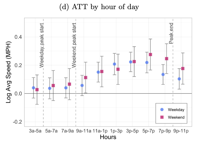
Example: effects of congestion pricing in NYC

Even though only NYC implemented congestion pricing, average speeds in most cities increased in January and February. To get a better counterfactual, they used a synthetic control formed from other cities. They found a significant ATT (15%) on daily and hourly average speed.

Example: effects of congestion pricing in NYC

The effect is mainly within and to CBD, although small increases in speed of 4% can be seen on trips to other areas that go through the CBD.

Example: effects of congestion pricing in NYC

Using CATE, they also investigate the effect across different groups. They found similar effects across the income distributions.

Example: effects of congestion pricing in NYC

Summary:

• Use of Google Maps Traffic Trends to get the travel times and speeds for different routes to and within CBD.
• Effect of congestion pricing was confounded by increase of average speeds also in other cities.
• Use of other cities as donors for a synthetic control.
• ATT is around 15%, compared with the raw 18%.
• Thus, most of the change in average speed is then attributable to the policy.
• Use of CATE to investigate effect across demographic groups. They found no significant difference across the income distribution.

Example: measuring the impact of slow zones on street life using social media

In the early 2000s, Paris began to promote sustainable transport models. The Paris Pedestrian Initiative implemented a street-sharing program to promote alternative modes of transportation (bikers, pedestrians). A key component of this program was the Zone 30 initiative to create slow zones.

Example: measuring the impact of slow zones on street life using social media

To do that they fixed the speed limit of 30km/h, created more space for bikes, sidewalks, and parking space was converted to terraces in some streets.

Example: measuring the impact of slow zones on street life using social media

There were 141 slow zones introduce in Paris, located within the central area of Paris and implemented across ten years.

Example: measuring the impact of slow zones on street life using social media

One of the key components of this policy is its implementation: it was done at the level of the district, which means that streets outside of those slow zones were not affected by the policy. This was used by Salazar-Miranda et al. [2] to evaluate the impact of policy using causal methods.

They define treated streets as those within slow zones and control as those 100m or less from the boundary of slow zones.

Example: measuring the impact of slow zones on street life using social media

Their choice of treated and control groups was made to maximize their similarity across all other potential confounders like length, proximity to the city center, transit stops, parks, etc., that might affect the outcome of the policy. They only found differences in segment length, thus they control for it later.

Example: measuring the impact of slow zones on street life using social media

Outcome: do slow zones affect human activity on streets?

• To measure it, they used geolocalized tweets from Twitter from 2010 to 2015
• They collected 10.5M geotagged posts.
• They aggregated the number of tweets by streets.
• They hypothesize that if slow zones attract more people, there will be more tweets there.
• However, they are probably measuring too how “tweetable” is the street, and the,s people visiting the street tweet more often when visiting.
• Thus, they look at the total number of tweets and the number of tweets per user.

Example: measuring the impact of slow zones on street life using social media

First: does human activity vary across the boundaries of slow zones? There appears to be a discontinuity in the regressions of activities across the boundaries. This justifies their choice of control and treatment groups.

Example: measuring the impact of slow zones on street life using social media

They used a similar framework as regression discontinuity to measure the ATE by investigating the average effect of segments of a street that are at different sides of the slow zone boundary:

\[ Outcome_{i,t} = \beta\ SlowZone_{i,t} + \gamma\ X_i + \delta_t + \alpha_{n(i)} + \theta_{s(i)} + \epsilon_{i,t} \]

where

• \(SlowZone_{i,t}\) is an indicator equal to 1 if the street segment lies within a slow zone at time \(t\).
• \(X_i\) is a vector of covariates of the street (including the street length).
• \(\delta_t\) are year-fixed effects
• \(\alpha_{n(i)}\) denotes neighborhood fixed effects
• \(\theta_{s(i)}\) denotes street fixed effects. It ensures that we are correctly comparing street segments that are part of the same street.

Example: measuring the impact of slow zones on street life using social media

They claim that, since control and treated segments of the same street at different sides of the boundary are significantly different in terms of characteristics (apart from the street length), then \(\beta\) can be interpreted as the causal impact. Here are the results for different outcomes (44% increase in the number of tweets!)

Example: measuring the impact of slow zones on street life using social media

However, they found that the effect is only significant for early cohorts (2010) of slow zones. Probably because of under-powered statistical analysis

Example: measuring the impact of slow zones on street life using social media

Summary:

• Using geotagged Tweets and a discontinuity regression framework, they show that the slow zones initiative increased human activity by 44%
• However, the effect is not significant for late cohorts of slow zones.
• They do not control for potential spillovers.
• Neither did they implement a DiD design in their regressions.
• Also, Twitter activity can measure different outcomes from the ones the policy was meant to achieve: walkability, fewer cars, and more commercial activity.

Example: effects of EV charging stations on business

Electric Vehicles (EVs) offer a possibility to alleviate the problem of pollution in our cities. Some policies, like the Infrastructure Investment and Jobs Act (IIJA) in 2021 ($7.5B) promote the creation of public EV charger stations (EVCS) across the nation.

However, the importance of public EVCSs extends beyond their primary function: they can influence the economic outcomes of surrounding businesses. Does the foot traffic around EVCS boost or harm those businesses?

Example: effects of EV charging stations on business

In a recent paper [3], Zheng et al. investigate this through causal methods

• They analyze data from over 4000 EVCS and 140,000 businesses in California from 2019 to 2023.
• They investigate the increase in the foot traffic of businesses around EVCS.
• Foot traffic data comes from Safegraph.
• Because EVCS are not randomly created, they control for self-selection and omit variable biases in different ways: propensity matching, DiD, and event study.

Example: effects of EV charging stations on business

Their data includes when a charging station is opened. They considered that all POI locations within a 500m during the study period are part of the treatment group. Control are POI locations outside that 500m boundary.

Example: effects of EV charging stations on business

One limitation of that approach is that ECVS provides might place them strategically to maximize the benefits of them, in areas that could have more growth, for example. To address this endogeneity, the authors use Propensity Score Matching to pair same-category POIs in the treatment and control group.

This is done using logistic regression. Let’s assume that \(D_i\) is the treatment for POI \(i\) and \(X_i\) are observable covariates that might influence the probability that \(i\) is treated

\[ logit P(D_i = 1|X) = \beta_0 + \beta_1 X_1 + \cdots +\beta_k X_k \] \(P(D_i = 1 | X)\) is called the propensity score. The matching is very simple: for each treated unit, we found a control unit with a similar score.

Example: effects of EV charging stations on business

Once this is done, typically, we should observe that the distribution of covariates between treated and control groups should be similar

Example: effects of EV charging stations on business

Using that matched sample of control and treated POIs, they look at different outcomes, like customer count, spending, etc.

To get the ATE, the use a DiD:

\[ \ln Y_{it} = \alpha + \beta D_{it} \times PC_{it} + u_i + \phi_c \times \omega_t + \epsilon_{it} \] where

• \(D_{it}\) is the treatment, \(D_{it}=1\) if an EVCS was opened beforethe time \(t\) and located within 500 of POI \(i\)
• \(PC_{it}\) is the total count of charging ports at an EVCS opened until \(t\) within 500 of POI \(i\).
• \(u_i\) denotes POI fixed effects
• \(\phi_c \times \omega_t\) are county \(\times\) time fixed efects.

\(\beta\) is then the marginal effect of adding a new charging port to an EVCS.

Example: effects of EV charging stations on business

They found that adding a new charging port resulted in a 0.21% increase in customer count and a 0.25% in spending in 2019 and 0.14% and 0.16% in 2021-2023.

Example: effects of EV charging stations on business

The effect is very small (!!) and has some demographic, temporal, and spatial heterogeneity. For example, they found that for underprivileged regions, the effect was 0.17%/0.29% in 2019 and that the effect diminishes with distance to EVCS and does not increase with time.

Example: effects of EV charging stations on business

They also found some differences across categories. Only Restaurants and Grocery/clothing stores seem to be affect (and only for fast chargers)

Example: effects of EV charging stations on business

Summary:

• EVCS have an impact on the business around. However, the impact is small and only concentrated in close POIs from some categories.
• To minimize potential bias in the selection of places to install EVCS, the authors used Propensity Score Matching.
• However, they didn’t account for potential spill-overs by doing a placebo test. Given the small effect found, it is highly likely that the effect might not be significant when using a placebo test.

Conclusions

• Most policy evaluations are flawed when they rely on simple before-after comparisons or ignore spatial complexity, selection bias, and spillovers.
• Causal inference is essential to move from correlation to robust, actionable insights — especially in complex, dynamic urban systems.
• Computational Urban Science offers new opportunities to evaluate policies at scale, in real-time, and with fine spatial and demographic resolution.
• Big data is not enough without sound methodological design, large-scale datasets can mislead rather than inform.
• Better policy needs better evidence. CUS allows us to ask: Did the policy work? For whom? Where? Why? And what happened around it?

Further reading

• Causal Inference: The Mixtape Book by Scott Cunningham
• Causal Inference for the Brave and True by Matheus Facure. He is the author of the book Causal Inference in Python
• Econometric methods for Program Evaluation by Abadie et al. [4]
• Spatial Causality: a systematic review on Spatial Causal Inference, by Akbar et al. [5]

References

[1]

C. Cook et al., “The Short-Run Effects of Congestion Pricing in New York City.” in Working Paper Series. National Bureau of Economic Research, Mar. 2025. doi: 10.3386/w33584.

[2]

A. Salazar-Miranda, C. Heine, F. Duarte, K. Schechtner, and C. Ratti, “Measuring the impact of slow zones on street life using social media,” Cities, vol. 131, p. 104010, Dec. 2022, doi: 10.1016/j.cities.2022.104010.

[3]

Y. Zheng, D. R. Keith, S. Wang, M. Diao, and J. Zhao, “Effects of electric vehicle charging stations on the economic vitality of local businesses,” Nature Communications, vol. 15, no. 1, p. 7437, Sep. 2024, doi: 10.1038/s41467-024-51554-9.

[4]

A. Abadie and M. D. Cattaneo, “Econometric Methods for Program Evaluation,” Annual Review of Economics, vol. 10, no. 1, pp. 465–503, Aug. 2018, doi: 10.1146/annurev-economics-080217-053402.

[5]

K. Akbari, S. Winter, and M. Tomko, “Spatial Causality: A Systematic Review on Spatial Causal Inference,” Geographical Analysis, vol. 55, no. 1, pp. 56–89, 2023, doi: 10.1111/gean.12312.