Beyond the “what”
So far, we have seen methods to understand urban data, describe it, and predict it.
Statistical methods, including Machine Learning, are very useful in answering questions about the “what” and the “how much.”
Causes and effects are a different story. Causal inference is about answering the “why” by studying the “what if”
![]()
“for every question you can think of, there is an answer that is simple, intuitive, and wrong.”
Beyond the “what”
And the reason is that associations (correlations) can be deceiving.
![]()
From Andreas Raaskov
We can associate them, and even use drownings to predict ice cream. \[
\text{icecream}_t = \beta_0 + \beta_1 \text{drownings}_t + \epsilon_t
\] \[
\text{icecream}_{t+1} = \beta_0 + \beta_1 \text{drownings}_t + \epsilon_t
\]
The “why”
The fundamental question of causal inference is to understand why things happen, or more specifically if a change in one variable causes a change in another. For example:
- Will this change in a bus line increase the number of people taking the bus?
- Does the opening of a new supermarket increase the number of people visiting the restaurants in the area?
To answer these questions, we need to design experiments that allow us to isolate the effect of a change in one variable on another.
The idea is very simple but impossible: take the same city with the same people, create two universes, one with the change (treatment) and one without it, and compare the results (outcome).
Brief Intro to Causal Inference
Brief Intro to Causal Inference
Units: To keep it simple, assume we have different units \(i\). Those units can be cities, people, or any other entity. For example, they could be the people in a city who consume food in restaurants.
Outcome: we want to study the effect of a cause on a particular outcome for those units \(Y_i\), like the number of people consuming fast food.
Experiment: to understand the effect of a cause (e.g., a new SNAP program to consume healthy food), we design experiments in which we give people the treatment (access to the program) \(T_i = 1\) or not \(T_i = 0\).
Causal model. OUr idea is to investigate the causal link between treatment and outcome.
![]()
Potential vs. realized outcomes
Before the intervention, units have potential outcomes:
- \(Y_{0i}\) if unit \(i\) does not receive the treatment \(T_i = 0\) and
- \(Y_{1i}\) if unit \(i\) does receive it \(T_i=1\).
Note, however, that only one of them is realized. Thus, we have one potential outcome and one realized outcome. They are related like this:
\[
Y_i = T_i Y_{1i} + (1-T_i) Y_{0i}
\]
This is a critical equation, showing that we can never observe both potential outcomes for the same unit.
If \(i\) received the intervention, \(Y_{1i}\) is the realized outcome and \(Y_{0i}\) is the counterfactual outcome.
Causal Effect
The causal effect of the treatment on the outcome is defined as the difference between the potential outcomes (we will use the notation \(^*\) for those values which are potential)
- At individual level \[
\text{ITE}^*_i = Y_{1i} - Y_{0i}
\]
- Or aggregated level over the units \[
\text{ATE}^* = \mathbb{E}[Y_{1i} - Y_{0i}]
\]
- Or aggregated treatment effect on the treated \[
\text{ATT}^* = \mathbb{E}[Y_{1i} - Y_{0i}|T_i=1]
\]
Causal effect
Note that ITE/ATE/ATT can not be calculated by observing the intervention, as we can only observe one of the potential outcomes.
This is called the fundamental problem of causal inference, since we cannot observe the counterfactual outcome for each individual. In our case, we cannot observe the consumption of fast-food by an individual if they did or did not have access to the SNAP program at the same time.
One tempting way to estimate the causal effect is to compare the outcomes of the treated and untreated units. This is called the naive estimator:
\[
\text{ATE} = \mathbb{E}[Y_i|T_i=1] - \mathbb{E}[Y_i|T_i=0]
\]
However, this is not the causal effect, as the difference between the two groups might be due to other factors, like the fact that people who are more likely to consume fast-food are also more likely to enroll in the SNAP program.
SUTVA
Although everything we said so far makes sense, there is a number of important assumptions we did so far. The most critical one is the Stable Unit Treatment Value Assumption (SUTVA) which is underneath the equation \(Y_i = T_i Y_{1i} + (1-T_i) Y_{0i}\).
This assumption consists of two other sub-assumptions:
- No interference: the potential outcome of one unit does not depend on the treatment of another unit. That means there are no spillovers or interferences between the outcomes of different units.
- No hidden variations of treament: for each unit there are no different forms of the treatment. That is, the treatment is the same for all units.
SUTVA, Violations in Urban Problems
Both assumptions are critical, and in many cases, they are not met in urban problems:
In urban areas, businesses or individuals might be affected by the treatment given to other people due to the interconnectedness of activities, transportation, or policies in cities. That is, in urban areas, where social behavior contagion, communication, or transportation between areas is important, we have to pay special attention to spillovers or interference between units.
Similarly, in urban areas, treatments are typically variable. For example, consider the complex policy implementation to create new businesses in urban areas. Even though the policy (e.g., tax reduction) is the same, some districts might have implemented it with different durations, extending or giving the potentially affected population different information.
Experimental Causal Inference
Solving the causal inference problem
One tempting way to estimate the causal effect is to compare the outcomes of the treated and untreated units. This is called the naive estimator:
\[
\text{ATE} = \mathbb{E}[Y_i|T_i=1] - \mathbb{E}[Y_i|T_i=0]
\]
However, this is not the causal effect, as the difference between the two groups might be due to other factors, like the fact that people who are more likely to consume fast-food are also more likely to enroll in the SNAP program.
Is there a way to make sure that \(\text{ATE} = \text{ATE}^*\)?
Solving the causal inference problem
Before that, let’s investigate why \(\text{ATE}\) and \(\text{ATE}^*\) are different. First we note that
\[
\mathbb{E}[Y_i | T_i = 1] = \mathbb{E}[Y_{1i} | T_i = 1], \quad \mathbb{E}[Y_i | T_i = 0] = \mathbb{E}[Y_{0i} | T_i = 0]
\] That is, the average of realized outcomes of the treated/control units is equal to the average of the potential outcomes of the treated/control units.
Summing and subtracting \(\mathbb{E}[Y_{0i}|T_i=1]\) into that equation ,we get the following important result that ATE can be divided into two components
\[
ATE = \underbrace{\mathbb{E}[Y_{1i}|T_i=1] -\mathbb{E}[Y_{0i}|T_i=1]}_{\text{ATT*, Average treatment effect on the treated}} + \underbrace{\mathbb{E}[Y_{0i}|T_i=1]- \mathbb{E}[Y_{0i}|T_i=0]}_{\text{Selection bias}}
\] Thus, the difference between the observed \(\text{ATE}\) and the potential \(\text{ATT}*\) is the selection bias which measures the difference between the potential outcomes of the treated and untreated units.
Solving the causal inference problem
How can we remove the selection bias? The best way is to perform an A/B experiment and randomize the treatment among units. That is, to assign the treatment randomly to the units. In that case, the average potential outcome of all units after treatment is the average over the realized outcome of units that received the treatment
\[
\mathbb{E}[Y_{1i}] = \mathbb{E}[Y_{1i}|T_i=1]
\]
and the same for the control group.
\[
\mathbb{E}[Y_{0i}] = \mathbb{E}[Y_{0i}|T_i=0]
\]
Solving the causal inference problem
This has two consequences:
The first one is that the \(ATE\) and \(ATE^*\) coincide because \[
ATE^* = \mathbb{E}[Y_{1i}-Y_{0i}] = \mathbb{E}(Y_{1i}) - \mathbb{E}(Y_{0i}) = \mathbb{E}(Y_{1i}|T_i=1) - \mathbb{E}(Y_{0i}|T_i=0) = ATE.
\]
The second one is that the selection bias is zero, as the treatment is randomly assigned and thus the \(ATE^*\) is equal to the \(\text{ATT}*\).
Solving the causal inference problem
One word of caution:
The equivalence of \(\text{ATE}^*\) and \(\text{ATE}\) is only on average. This means that we can estimate the average treatment effect for large experiments.
In small experiments, we might still have a selection bias, and the \(\text{ATE}\) might not be equal to the \(\text{ATE}^*\).
Also, in general, \(\text{ATE}^*\) has error bars, and we need to estimate the uncertainty of the causal effect.
All you need is regression
A good way to investigate the ATE and its statistical uncertainty is by using regressions. If we take all the outcomes of our units \(Y_i\) and regress them on the treatment \(T_i\) we can estimate the ATE as the coefficient \(\beta_1\) of the treatment in the regression.
\[
Y_i = \beta_0 + \beta_1 T_i + \epsilon_i
\]
We typically measure \(\beta_1\) as the average treatment effect (ATE) and its standard error as the uncertainty of the ATE. Its p-value will give us an indication of how likely it is that the treatment has an effect.
All you need is regression
To estimate the effect size, we can normalize the ATE by the average of the outcome of the control group. This is called the effect size. One simple way to estimate the effect size is to divide the ATE by the control group’s average.
\[
\text{Effectsize} = \beta_1 / \mathbb{E}[Y_i | T_i=0]
\]
Another typical way is to regress the \(\log\) of the outcome \[
\log Y_i = \beta_0 + \beta_1 T_i + \epsilon_i
\]
In that case we get \[
\text{Effectsize} = \exp(\beta_1) - 1 \simeq \beta_1
\] if \(\beta_1\) is small.
Conditional ATE
The ATE can be different for different groups of units. For example, the SNAP program’s effect might differ for different income groups. In that case, we can estimate the ATE for each group of units. This is called the conditional ATE.
To estimate the conditional ATE, we can include an interaction term between the treatment and the group in the regression
\[
Y_i = \beta_0 + \beta_1 T_i + \beta_2 X_i + \beta_3 T_i X_i + \epsilon_i
\]
The coefficient \(\beta_3\) give us how treatment effects change with \(X_i\)
Confounders
In many cases, and especially in urban areas, the treatment is not randomly assigned. For example, the people who participated in the SNAP program might be from low-income groups, and thus, our results might be affected by the different impacts of the treatment across income groups. Also, groups of different incomes might have different outcomes in the program under the same treatment.
A variable affecting both the treatment and the outcomes is a confounder.
![]()
Confounders
Confounders can bias our estimate of the ATE; thus, we have to consider them in our analysis. In that case, we can include those variables in the regression:
\[
Y_i = \beta_0 + \beta_1 T_i + \beta_2 X_i + \epsilon_i
\]
where \(X_i\) are the confounders. The coefficient \(\beta_1\) will then give us the ATE, controlling for the confounders.
This is because in a linear regression, the coefficient \(\beta_i\) is the bivariate coefficient of the same regressor after accounting for the effect of other variables in the model (see Causal Inference for the Brave and True)
Quasi-experimental Causal Inference
Quasi-experimental Causal Inference
Quasi-experimental methods are statistical techniques used to estimate causal effects when randomized controlled trials (RCTs) are not feasible. Unlike experiments, where treatment is randomly assigned, quasi-experiments rely on observational data and exploit natural variations to define those groups, control for unobserved confounders and infer causality.
These methods aim to mimic randomization using statistical techniques that control for observed or unobserved confounders and establish a credible counterfactual (i.e., what would have happened without the treatment).
- Propensity score matching
- Instrumental Variables
- Regression discontinuity
- Difference in Differences
- Synthetic Control
Propensity score matching
Propensity score matching is used to estimate the average treatment effect (ATE) in observational studies, where randomization is not possible. The idea is to match treated and untreated units based on their propensity score \(P(T_i=1 | X)\), which is the probability of receiving the treatment given the observed covariates.
- First, we model \(P(T_i=1 | X_i)\) using a logistic regression.
- Then we match each treated unit with an untreated unit with a similar propensity score.
- Finally, we estimate the ATE by comparing the outcomes of the matched treated and untreated units.
However, it only controls for observed confounders. Unobserved confounders can still bias the estimate.
Propensity score matching
Example: study the adoption of an offline behavior of attending a cultural event by social influence. Matching done using mobility characteristics of people [2]
![]()
Propensity score matching using mobility data, from [2]
Instrumental variables
Instrumental variables (IV) is a method used to estimate the causal effect of a treatment \(T\) on an outcome \(Y\) when there is unobserved confounding. The idea is to find a variable \(IV\) that affects the treatment but not the outcome directly. This variable is called an instrumental variable.
![]()
Instrumental variables
For example, the effect of education on earnings can be estimated using distance to school as an instrumental variable. Distance to school is related to education but not to earnings directly.
The causal effect is obtained through a Two-Stage Least Squares (2SLS):
- Regress the treatment on the instrumental variable to estimate the effect of the treatment on the outcome, \(\hat T_i = \beta_0 + \beta_1 IV_i + \varepsilon_i\).
- Regress the predicted treatment outcome from the first stage to estimate the causal effect. \(Y_i = \alpha_0 + \alpha_1 \hat T_i + \varepsilon_i\).
- If the instrumental variable is valid, the coefficient \(\alpha_1\) will give us the causal effect.
Instrumental variables
Example: using family or friend links as instrumental variables to estimate the effect of social influence on economic flows in urban areas [3]
![]()
Using family and friend connections to understand the effect of social influence on economic flows, from [3]
Regression discontinuity
Regression discontinuity (RD) is a method used to estimate the causal effect of a treatment on an outcome when the treatment is assigned based on a threshold. The idea is to compare the outcomes of units just above and below the threshold. This way, we can estimate the ATE for the units affected by the treatment.
Example: studying the effect of a policy on businesses in a city by comparing the outcomes of businesses that are just above and below the policy’s threshold.
This is typically done by running two regressions:
- One for the units just above the threshold and one for those just below the threshold.
- The difference in the coefficients of the two regressions gives us the causal effect.
Regression discontinuity
Example: using regression discontinuity and social media data to study the impact of slow zones (areas where speed limits are reduced) on human activity on streets [4]
![]()
Using regression discontinuity to study the impact of slow zones on human activity, by [4]
Difference-in-differences
We often have panel data, observing the same units over time. In that case, we can use difference-in-differences (DiD) to estimate the causal effect of a treatment on an outcome.
In DiD, we compare the changes in the outcomes before and after the treatment for the treated and untreated units. This way, we can estimate the ATE for the units affected by the treatment.
The assumption of the difference-in-differences is that the outcome trend for the treated and untreated units would be the same if the treatment were not applied. This is called the parallel trends assumption.
Thus, any confounding factor is time-invariant and similarly affects the treated and untreated units. Let’s call \(P_t=0\) the post and \(P_t=1\) pre-treatment periods. The parallel trends assumption is that:
\[
\mathbb{E}[Y_{0it}|T_i=1,P_t=1] - \mathbb{E}[Y_{0it}|T_i=1,P_t=0] =
\] \[
\mathbb{E}[Y_{0it}|T_i=0,P_t=1] - \mathbb{E}[Y_{0it}|T_i=0,P_t=0]
\]
Difference-in-differences
Note that even if there would have been no treatment/experiment, we could still have a change in the variable outcome due to other confounding variables or covariates.
For example, if we want to implement a public transportation policy in an urban area to change the car usage in that area, we might still consider the possibility that gas prices might change car usage throughout the whole city.
The parallel trends assumption means that if we do not intervene, that covariate (gas prices) might affect both the treatment and control areas similarly. How plausible is the parallel trends assumption depends greatly on our problem and our knowledge of potential covariates that might explain the effect of intervention.
Difference-in-differences
As before, the effect of the intervention is estimated by the \(ATT^*\) in the post-treatment period.
\[
ATT^*[P_t=1] = \mathbb{E}[Y_{1it}|T_i = 1, P_t=1] - \mathbb{E}[Y_{0it}|T_i = 1, P_t=1]
\]
Using the equation above and reordering we get \[
\begin{eqnarray}
ATT^*[P_t=1] &=& \mathbb{E}[Y_{1it}|T_i = 1, P_t=1] - \mathbb{E}[Y_{0it}|T_i=0,P_t=1] \\
& & - (\mathbb{E}[Y_{0it}|T_i=1,P_t=0] - \mathbb{E}[Y_{0it}|T_i=0,P_t=0]),
\end{eqnarray}
\] This means that the average treatment can be expressed as a difference of differences: the first difference is the difference between outcomes in the treated and control groups after the treatment. The second one is the difference between the outcomes of those groups before the treatment.
Difference-in-differences
![]()
DiD
Difference-in-differences
As before we can estimate ATT* using a regression
\[
Y_{it} = \beta_0 + \beta_1 P_t + \beta_2 T_i + \beta_3 P_t \times T_i + \gamma X_{it} + \varepsilon_{it}
\] where \(X_{it}\) are the confounders (they cannot violate the parallel trends hypothesis, i.e they have to affect both treated and control groups similarly). The coefficient \(\beta_3\) will then give us the ATT*.
![]()
DiD
Synthetic Control
Another way to estimate panel data’s causal effect is using the synthetic control method (SCM). The key idea is to create a synthetic control group that mimics the treated group before the treatment. This is done by combining a weighted average of the control units.
Although SCM can be done for many treated units, it is typically used for a single treated unit. Let’s assume that it is the \(i=1\) and the rest \(i = 2,\ldots,N\) are controls or donors to the synthetic control. If the intervention happens at the time \(T\), the SCM is estimated by
\[
Y_{1t} \simeq \sum_{i=2}^N w_i Y_{it}
\]
Synthetic Control
The weights \(w_i\) are chosen to minimize the difference between the treated and synthetic control group before the treatment.
\[
\text{min}_{\sum w_j=1, w_j\geq0} \sum_{t=1}^{T} \left( Y_{1t} - \sum_{j \in \text{Donors}} w_j Y_{jt} \right)^2
\]
Since we typically have one treated unit and many donors, to prevent overfitting, the weights are typically constrained to be non-negative and sum to one. There are other options, like LASSO.
Synthetic Control
The causal effect can be estimated using DiD on the treated and synthetic control group after the treatment.
Note by definition, the synthetic control incorporates the parallel trends assumption, as it is constructed to match the treated unit before the treatment.
![]()
SCM
Synthetic Control
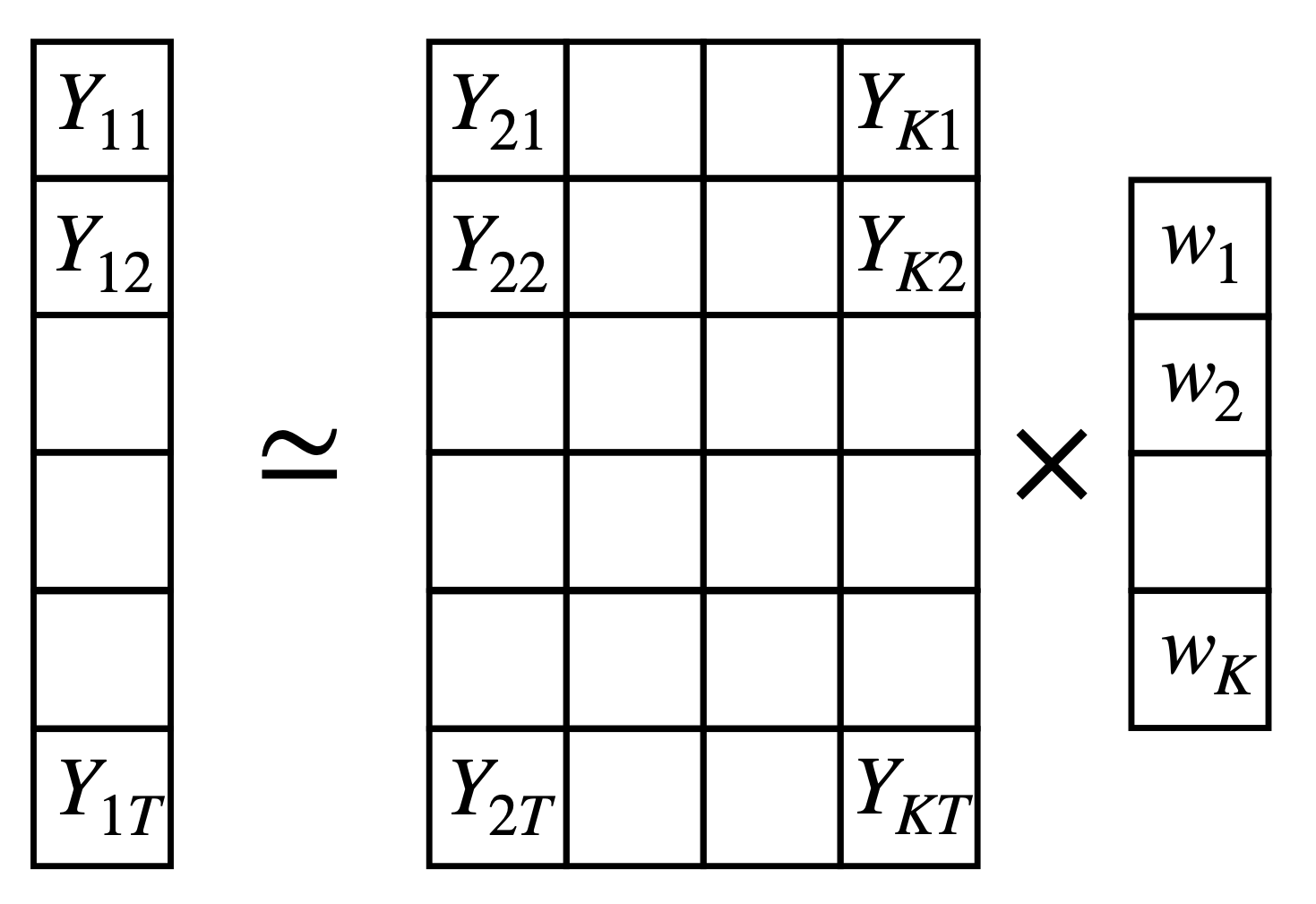
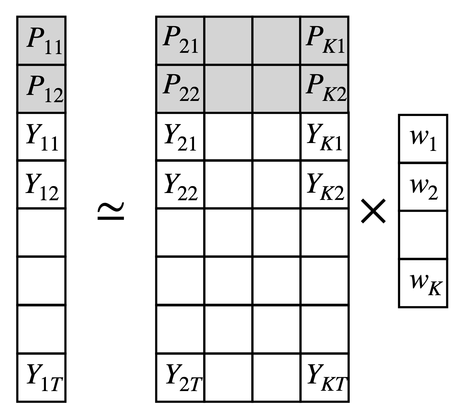
The synthetic control method can be written as a matrix equation
\[
min_{||w|| = 0, w_\geq 0 } ||y - Xw||^2
\]
where \(y\) is the outcome of the treated unit, \(X\) is the matrix of outcomes of the control units and \(w\) is the vector of weights. The vectors \(y\) and matrix \(X\) can be extended to include confounders or predictors.
Synthetic Control
Use other states as donors to estimate the effect of tobacco control policies in California (proposition 99) on smoking rates [5]
![]()
SCM for tobacco control policies in California