library(tidyverse)
library(arrow)
library(sf)Homework 1 - 15-minute cities in the US
Objective
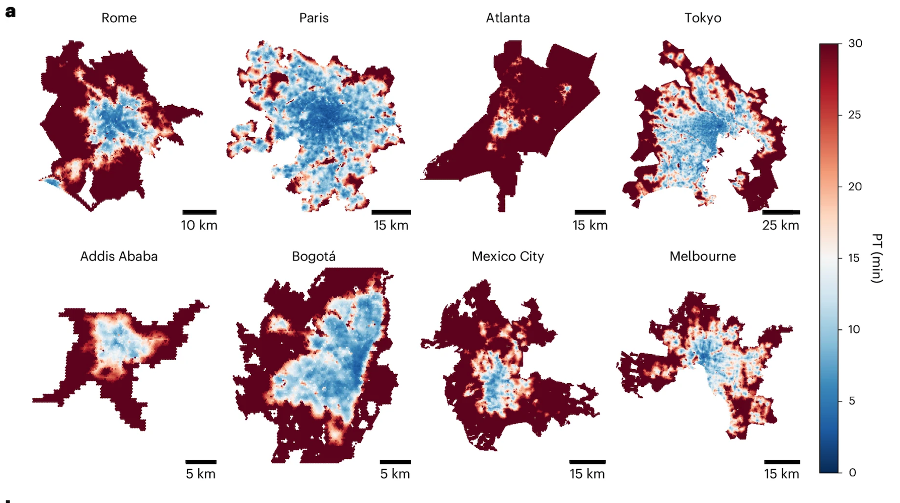
In this homework, we will explore the concept of the 15-minute city in the US. The 15-minute city is a concept popularized by the mayor of Paris and has been adopted by many cities worldwide. The idea is to create cities where people can access all the services they need within a 15-minute walk or bike ride from their homes. In this homework, we will explore how close the different areas in the US are to achieving this goal by analyzing data on the distribution of services in US cities.
There are different dimensions to the 15-minute city concept [1]. One dimension is the distribution of services such as grocery stores, restaurants, schools, parks, or transportation. Another dimension is the distribution of jobs and housing. In this homework, we will focus on the distribution of services in US cities.
Methodology
The objective of the HW is to find out which demographic groups within areas in the US are to achieve the 15-minute city goal. Here are the instructions
- Geographical context: Each student should focus on a particular Metropolitan area.
- Data: Use the Foursquare Open POI dataset to extract the location of Points of Interest (POIs) in that area.
- Data: Use the Census ACS tables to get the demographic characteristics of each Census Block Group (CBG) in that area.
- Calculating accessibility
- For each CBG \(k\) in that area, calculate the distance to the nearest 20 POIs of the category \(c\), \(t_{i}^{k,c}\).
- Use those distances to create a measure of the “accessibility” of each CBG to all services in the area (see, for example, [1]).
- Justify your choice of that metric of accessibility. You can also choose a binary variable of accessibility, which measures if the average time to the top 20 POIs of a category is within 15 minutes.
- To convert between distance and time, use the average speed of walking or biking in the US.
- Models
- Model the average accessibility of each CBG as a function of the demographic characteristics of that CBG using spatial linear regressions. Control for potential spatial autocorrelation.
- Find the CBGs that are the farthest from achieving the 15-minute.
Submission
The submission should be a Jupyter/Quarto/RMarkdown notebook that includes the following sections:
- Introduction: A brief introduction to the concept of the 15-minute city and the objective of the homework.
- City: The name of the city you focus on and some context about it.
- Data: A description of the data you are using and how you are processing it.
- Calculating accessibility: A description of how you are calculating the accessibility of each CBG to services in the city.
- Modeling accessibility: A description of how you are modeling the accessibility of each CBG as a function of the demographic characteristics of that CBG.
- Results: A description of the results of your analysis, including the CBGs that are the farthest from achieving the 15-minute city goal.
- Conclusion: A brief conclusion summarizing the main findings of your analysis.
How to submit
- Produce the report in PDF format
- Put all your material (PDF + code used, NO DATA!!) in a zip code.
- Submit your zip code to Canvas.
Deadline: March 10th, 2025, 11:59pm
Grading
Total points available: 50
| Component | Points |
|---|---|
| Introduction, City, and Context | 5 |
| Data: preparation and preprocess | 5 |
| Calculating accessibility | 10 |
| Modeling accessibility | 10 |
| Results | 10 |
| Conclusion | 5 |
| Workflow & formatting | 5 |
Tips and help
Data
To calculate accessibility we need to use data on the distribution of services in US cities. We will use the data for the FourSquare Points of Interest (POIs) in the US. The data is available in the /data/CUS/FSQ_OS_Places/places directory in the Parquet format.
require(arrow)
files_path <- Sys.glob("/data/CUS/FSQ_OS_Places/places/*.parquet")
pois_FSQ <- open_dataset(files_path,format="parquet")
Let’s get the data for the Boston metro area:
boston <- pois_FSQ |>
  filter(country=="US" & (region=="MA" | region=="NH")) |>
  collect()
We only keep those POIs that have only a category
boston <- boston |>
  mutate(num_cat = map_int(fsq_category_labels, length)) |>
  filter(num_cat == 1)
Let’s put directly the category and parent category in the table
boston <- boston |>
  mutate(cat = map_chr(fsq_category_labels, ~.x[[1]]))
Get the parent category (the string before the first “>”)
boston <- boston |>
  mutate(parent_cat =  map_chr(cat, ~{
    trimws(sub("^(.*?)>.*", "\\1", .x))
  }))
This is the distribution of POIs by parent category
boston |> count(parent_cat)# A tibble: 10 × 2
parent_cat n
<chr> <int>
1 Arts and Entertainment 15881
2 Business and Professional Services 174143
3 Community and Government 63059
4 Dining and Drinking 57616
5 Event 2385
6 Health and Medicine 40338
7 Landmarks and Outdoors 38063
8 Retail 74620
9 Sports and Recreation 18039
10 Travel and Transportation 31931Calculating accessibility
Here we will use a very simple approach: accessibility to a category from a CBG is the average distance to the closest 20 POIs of that category from the centroid of the CBG.
Let’s load the data for all CBGs in the Boston area
cbgs <- st_read("/data/CUS/labs/6/14460_acs_2021_boston.geojson")Reading layer `14460_acs_2021_boston' from data source
`/data/CUS/labs/6/14460_acs_2021_boston.geojson' using driver `GeoJSON'
Simple feature collection with 3418 features and 66 fields
Geometry type: MULTIPOLYGON
Dimension: XY
Bounding box: xmin: -71.89877 ymin: 41.56585 xmax: -70.32252 ymax: 43.57279
Geodetic CRS: NAD83Let’s do it for the “Arts and Entertainment” category
cbgs_centroids <- cbgs |> select(geometry) |>
  st_centroid() |>
  st_coordinates()
pois_points <- boston |>
  filter(!is.na(longitude) & !is.na(latitude)) |>
  filter(parent_cat == "Arts and Entertainment") |>
  select(longitude, latitude)
Very simple way to calculate the distance from each CBG to the neareast 20 POIS. Note that the distance here is in degrees.
require(RANN)
nn <- RANN::nn2(pois_points, cbgs_centroids, k=20)
Calculate the average distance
cbgs <- cbgs |>
  mutate(avg_dist = rowMeans(nn$nn.dist))
Modeling accessibility
Simple OLS model
cbgs_model <- cbgs |>
  mutate(prop_bachelor = education.bachelor / age.total,
         prop_white = race.white / age.total,
         prop_employed = employment.civilian_employed/employment.civilian_labor_force,
         prop_home = trans.home/trans.total)
model <- lm(avg_dist ~ median_income + prop_bachelor + prop_white + prop_employed + prop_home,
data=cbgs_model)
summary(model)
Call:
lm(formula = avg_dist ~ median_income + prop_bachelor + prop_white +
    prop_employed + prop_home, data = cbgs_model)

Residuals:
      Min        1Q    Median        3Q       Max
-0.023782 -0.007021 -0.002010  0.004678  0.118790

Coefficients:
                Estimate Std. Error t value Pr(>|t|)
(Intercept)    4.934e-03  3.550e-03   1.390    0.165
median_income  1.075e-07  6.487e-09  16.567  < 2e-16 ***
prop_bachelor -3.376e-02  1.500e-03 -22.507  < 2e-16 ***
prop_white     2.280e-02  9.969e-04  22.873  < 2e-16 ***
prop_employed -5.599e-03  4.087e-03  -1.370    0.171
prop_home      2.235e-02  4.461e-03   5.011  5.7e-07 ***
---
Signif. codes:  0 '***' 0.001 '**' 0.01 '*' 0.05 '.' 0.1 ' ' 1

Residual standard error: 0.01129 on 3272 degrees of freedom
  (140 observations deleted due to missingness)
Multiple R-squared:  0.2727,    Adjusted R-squared:  0.2716
F-statistic: 245.4 on 5 and 3272 DF,  p-value: < 2.2e-16
References
[1]
M. Bruno, H. P. Monteiro Melo, B. Campanelli, and V. Loreto, “A universal framework for inclusive 15-minute cities,” Nature Cities, vol. 1, no. 10, pp. 633–641, Sep. 2024, doi: 10.1038/s44284-024-00119-4.