Lab 10-1 - Urban transportation network analysis

Author

Affiliations

Esteban Moro

Network Science Institute, Northeastern University

NETS 7983 Computational Urban Science

Objectives

In this lab, we will analyze the urban transportation networks using network analysis. We wil

• Retrieve an urban road network from OpenStreetMap using OSMnx.
• Analyze network properties with NetworkX.
• Visualize the network and key metrics.
• Explore network resilience through node removal simulations.

City Chosen: Boston, MA

Load some libraries and settings we will use

# !pip install osmnx
# !pip install networkx
# !pip install matplotlib
import osmnx as ox
import networkx as nx
import matplotlib.pyplot as plt
import numpy as np
import pandas as pd
import geopandas as gpd

ox.settings.use_cache = True

Load street networks

Let’s get the street network for Boston and save it for future access. Get also the speed and length of the edges.

place_name = "Boston, Massachusetts, USA"
G = ox.graph_from_place(place_name, network_type="drive")
G = ox.add_edge_speeds(G)
G = ox.add_edge_travel_times(G)
ox.save_graphml(G, filepath="/data/CUS/labs/10/boston_drive.graphml") #save it for future acccess

Load the street network from the previously saved file

G = ox.load_graphml("/data/CUS/labs/10/boston_drive.graphml")

Plot the network

fig, ax = ox.plot_graph(
  G, 
  node_size=.1, node_color="blue", 
  edge_color="#333333",edge_linewidth = 0.5,
  bgcolor="white")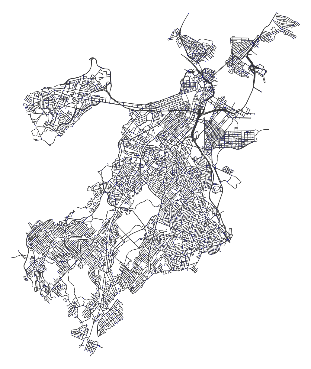

Road Network Analysis

Let’s analyze the road network properties

• Basic graph properties

print("Number of nodes:", G.number_of_nodes())
print("Number of edges:", G.number_of_edges())

Number of nodes: 11272
Number of edges: 25786

• Average node degree

avg_node_degree = np.mean([val for (node, val) in G.degree()])
print("Average node degree:", avg_node_degree)

Average node degree: 4.575230660042584

• Average edge length

avg_edge_length = np.mean([data['length'] for u, v, key, data in G.edges(keys=True, data=True)])
print("Average edge length:", avg_edge_length)

Average edge length: 100.52838481270976

• Average edge speed

avg_edge_speed = np.mean([data['speed_kph'] for u, v, key, data in G.edges(keys=True, data=True)])
print("Average edge speed:", avg_edge_speed)

Average edge speed: 40.710201825741315

• Degree distribution

degree_sequence = [d for n, d in G.degree()]
degree_counts = np.bincount(degree_sequence)
plt.figure(figsize=(8, 5))
plt.bar(range(len(degree_counts)), degree_counts, width=0.8, color="skyblue")
plt.title("Degree Distribution")
plt.xlabel("Degree")
plt.ylabel("Count")
plt.show()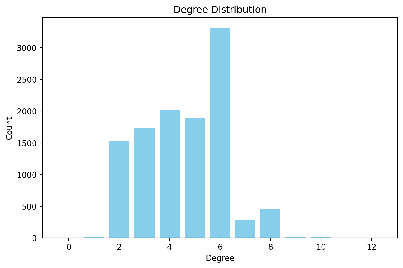

As we can see, contrary to other type of networks, nodes in road networks have very small degree.

• Clustering coefficient

clustering_coefficient = nx.average_clustering(ox.convert.to_digraph(G))
print("Clustering coefficient:", clustering_coefficient)

Clustering coefficient: 0.03012321164559398

As expected, the clustering coefficient is very low, as road networks are not clustered.

Note that road networks in osmnx are MultiDiGraphs, so we converted G_largest to a DiGraphs to calculate clustering (here) and centrality measures (see below).

Extract the largest strongly connected component (LSCC)

For metrics that require a strongly connected graph, we extract the LSCC.

G_largest = max(nx.strongly_connected_components(G), key=len)
G_largest = G.subgraph(G_largest).copy()
print("Number of nodes in the LSCC:", G_largest.number_of_nodes())
print("Number of edges in the LSCC:", G_largest.number_of_edges())

Number of nodes in the LSCC: 11192
Number of edges in the LSCC: 25644

Centrality Measures

Let’s calculate the betweenness centrality of the nodes in the LSCC. Calculating the centrality of each node is very expensive computationally, so we will calculate betweenness centrality for a subset of nodes (k=500).

bc = nx.betweenness_centrality(ox.convert.to_digraph(G_largest), weight="length",k=500)
max_node, max_bc = max(bc.items(), key=lambda x: x[1])
max_node, max_bc

(61341241, 0.14129948831440814)

As we can see, there is a node where a large fraction of the shortest paths pass through it.

Let’s look at the betweenness centrality of every node in the geographical space. Nodes with high centrality are in yellow and with low centrality in dark violet

nx.set_node_attributes(G_largest, bc, "bc")
gdf_nodes, gdf_edges = ox.graph_to_gdfs(G_largest)
nonzero_nodes = gdf_nodes[gdf_nodes["bc"] > 0.01]
fig, ax = plt.subplots(figsize=(10, 10))
gdf_edges.plot(ax=ax, linewidth=0.5, color="#333333", zorder=0)
nonzero_nodes.plot(ax=ax, markersize=5, column="bc", cmap="plasma", legend=True, zorder=1)
plt.title("Nodes with Nonzero Betweenness Centrality")
plt.show()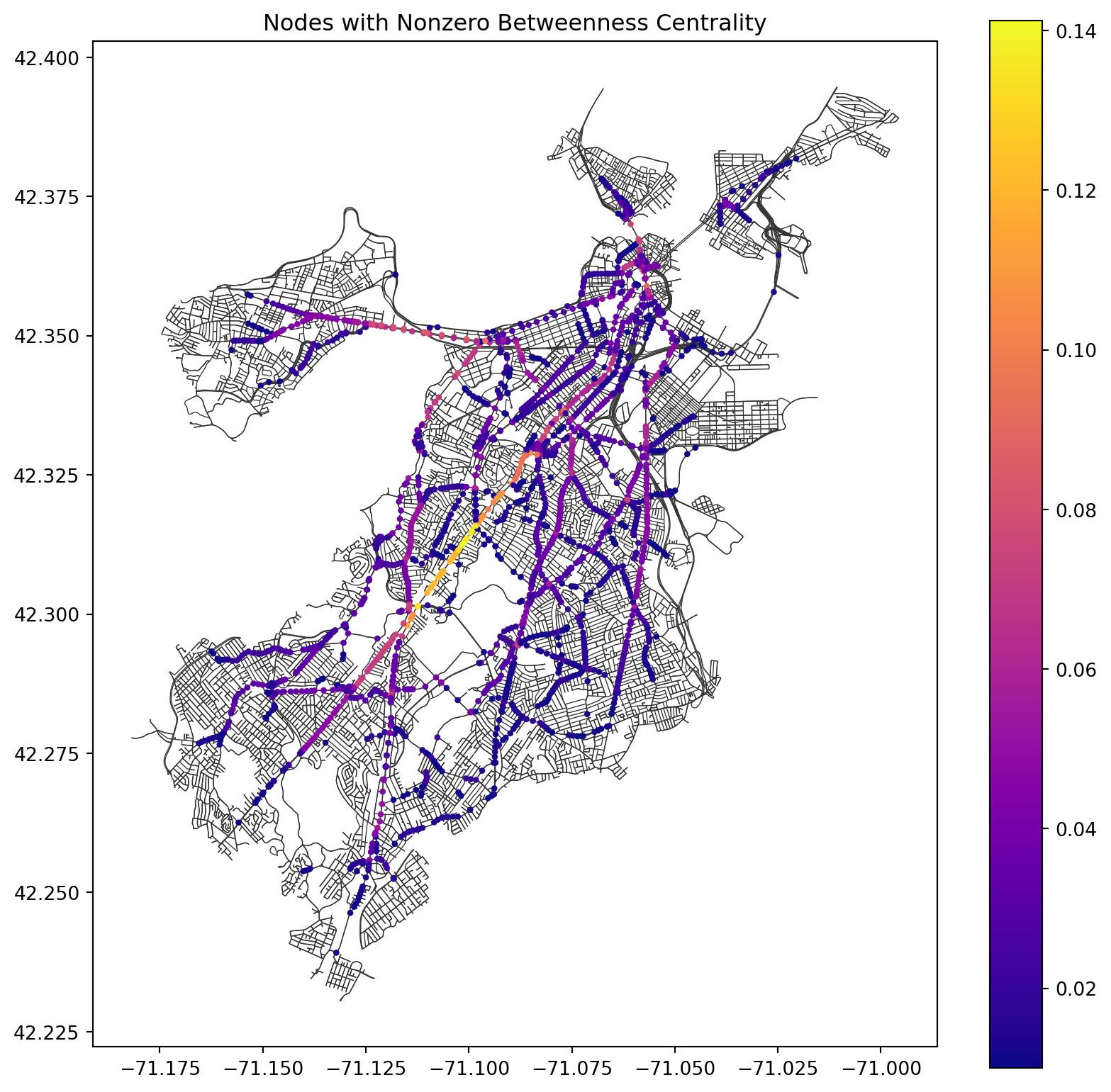

Network Resilience

Let’s analyze the network resilience by simulating node removals. We will remove nodes based on their betweenness centrality.

def simulate_node_removal(G, bc, n):
    G_copy = G.copy()
    nodes_to_remove = [node for node, _ in sorted(bc.items(), key=lambda x: x[1], reverse=True)[:n]]
    G_copy.remove_nodes_from(nodes_to_remove)
    return G_copy

Let’s simulate the removal of the 10% of the nodes with the highest betweenness centrality.

G_removed = simulate_node_removal(G_largest, bc, int(0.1 * G_largest.number_of_nodes()))
print("Number of nodes in the LSCC after removal:", G_removed.number_of_nodes())
print("Number of edges in the LSCC after removal:", G_removed.number_of_edges())
print("Size of the LSCC after removal:", len(max(nx.strongly_connected_components(G_removed), key=len)))

Number of nodes in the LSCC after removal: 10073
Number of edges in the LSCC after removal: 21726
Size of the LSCC after removal: 6745

Let’s do it for different fractions of nodes and plot the size of the LSCC after removal.

fractions = np.linspace(0, 0.5, 10)
lcc_sizes = []
for f in fractions:
    G_removed = simulate_node_removal(G_largest, bc, int(f * G_largest.number_of_nodes()))
    lcc_temp = max(nx.strongly_connected_components(G_removed), key=len)
    lcc_sizes.append(len(lcc_temp))

plt.figure(figsize=(8, 5))
plt.plot(fractions, np.array(lcc_sizes) / G_largest.number_of_nodes(), marker="o")
plt.xlabel("Fraction of Nodes Removed")
plt.ylabel("Size of Largest Connected Component")
plt.title("Network Resilience")
plt.show()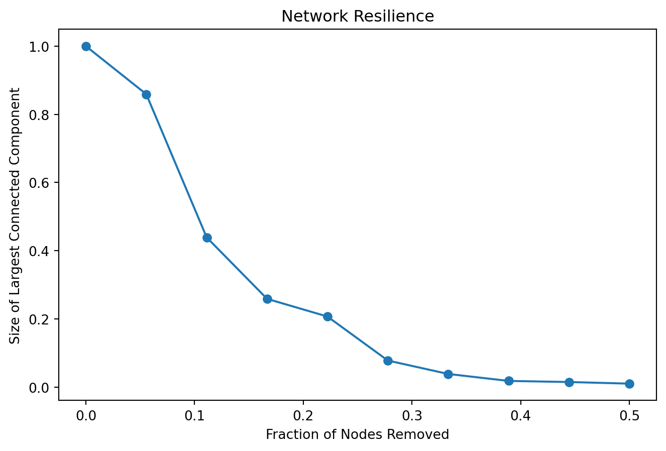

Your turn

In a recent paper [1], Boeing and Ha found that the resilience of road networks is related to different properties of the street network.

• Choose another street network in another city and calculate the network resilience. For example, use a city in other continent.
• Calculate the resilience of the street network and compare it with Boston.
• Which city has a more resilient street network to, e.g., 10% removal of nodes?
• What are the differences in the street network that make that city more/less resilient than Boston?

Conclusions

Road networks are different from other type of networks.

• They are planar graphs with low degree connectivity, low clustering
• Road networks tend to have high variability in centrality, which makes them fragile towards node removals.
• The resilience of road networks is then very dependent on the geography, interventions, and the city’s layout.

Further reading

• A review of the Structure of Street Networks by Barthelemy and Boeing

• Modeling and Analyzing Urban Networks and Amenities with OSMnx by Geoff Boeing

• Resilient by design: Simulating street network disruptions across every urban area in the world, by Boeing and Ha [1]

• Resilient urban forms: A review of literature on streets and street networks, by Sharifi [2]

References

[1]

G. Boeing and J. Ha, “Resilient by design: Simulating street network disruptions across every urban area in the world,” Transportation Research Part A: Policy and Practice, vol. 182, p. 104016, Apr. 2024, doi: 10.1016/j.tra.2024.104016.

[2]

A. Sharifi, “Resilient urban forms: A review of literature on streets and street networks,” Building and Environment, vol. 147, pp. 171–187, Jan. 2019, doi: 10.1016/j.buildenv.2018.09.040.