library(tidyverse)
library(arrow)
options(arrow.unsafe_metadata = TRUE)
library(DT) # for interactive tables
library(knitr) # for tables
library(ggthemes) # for ggplot themes
library(h3jsr) # for h3 hexagons
library(sf) # for spatial data
library(tigris) # for US geospatial data
library(Matrix) # for sparse matrices
theme_set(theme_hc() + theme(axis.title.y = element_text(angle = 90))) Lab 4-1 - Social media data
Relationship between mobility and social relationships
Objective
In this practical, we will use social media data to understand the relationship between social connections and geographical mobility. We will use the Gowalla dataset available at figshare which contains mobility and social relationships and mobility of users in the social network Gowalla
Specifically, we will:
- Understand the structure and multilayer nature of the data.
- Explore the data and understand the distribution of check-ins and social connections in urban areas.
- Analyze the relationship between social connections and mobility.
Load some libraries and settings we will use
Location-based social networks (LBSN)
LBSN are a type of social network that allow users to share their location and information about it. Similar to social networks, users can interact, message, and follow each other through the platform. The unique feature of LBSN is that users can share their location, find people nearby, or discover new locations.
The most popular geosocial networks are Yelp, Foursquare, Swarm, Facebook Places, and Gowalla. Although they were very popular in the early 2010s, they have lost popularity in recent years. For example, Foursquare recently closed down the Foursquare City Guide based on information about locations shared by its users. However, the data from these networks is still valuable for research purposes.
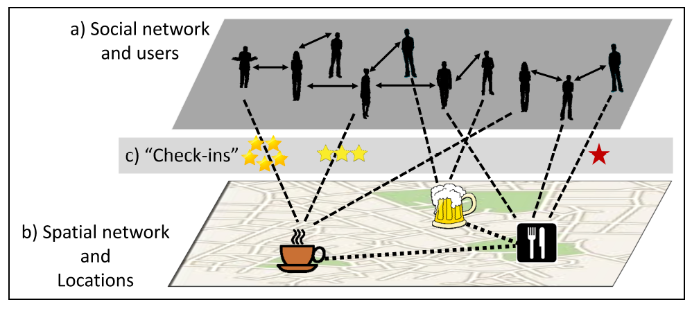
In LBSN we have information about:
- Users, the people using the platform.
- Places, the locations where users can check-in.
- Social interactions between the users, like interactions, follow, etc.
- Mobility patterns, the records of users moving from one place to another.
- Opinions and ratings about places, through the reviews and ratings users give to places.
This defines a complex hypergraph between users, places, and opinions.
Use of LBSN
LBSN were very popular among users, industry, and researchers.
Users can use the platform to find new places, share their location with friends, or discover new places. As we will see later, mobility and social connectivity are related, and users rely on their social connections to discover other places.
Business: understanding users’ mobility patterns can help businesses understand their customers’ behavior and design better marketing strategies. For example, businesses can use the data to understand the most popular places in a city, the most visited places, or the most popular places among a specific group of users. Businesses can also consider users’ check-ins to know the users’ opinions about their services.
Researchers can use the data to study human behavior, urban dynamics, or social networks. Although it cannot be used for current events in cities, researchers can use the data to test geo-social recommendation algorithms, study the relationship between social connections and mobility [1] [2], to understand the geographical structure of social networks.
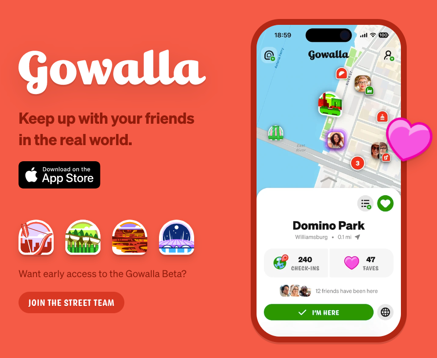
Gowalla
Gowalla was a location-based social network that allowed users to check in at places, share their location with friends, and discover new places. The platform was very popular in the early 2010s, but it was bought by Foursquare and closed down in 2012. It came back in 2023.

The data from Gowalla around 2010 is still available, and researchers use it to study human behavior, urban dynamics, and social networks. There are mainly two sources of Gowalla data:
- The SNAP repository at Stanford University contains a snapshot of the Gowalla network in 2010 from the [2] paper.
- The Figshare repository by Dingqi Yang contains a snapshot of the Gowalla network in 2010 and 2011.
If you are interested, there are other LBSN datasets available:
- Brightkite check-ins and social network
- Foursquare check-ins, including information about the places and social networks between users.
Gowalla Global-scale data
Let’s use the Figshare repository by Dingqi Yang, which you can find already in stella at the /data/CUS/gowalla folder
Check-ins
checkins <- open_dataset("/data/CUS/gowalla/gowalla_checkins.csv",
                         format="csv")
checkins |> head() |> kable()| userid | placeid | datetime |
|---|---|---|
| 1338 | 482954 | 2011-06-23 02:24:22 |
| 1338 | 580963 | 2011-06-22 14:23:03 |
| 1338 | 365256 | 2011-06-09 23:29:30 |
| 1338 | 89504 | 2011-05-22 15:54:30 |
| 1338 | 1267135 | 2011-05-21 16:51:13 |
| 1338 | 1487647 | 2011-05-16 18:40:41 |
Note that both the users and the places ids are anonymized. Here is the number of check-ins
dim(checkins)[1] 36001959 3Places visited
We also have the dataset of the places where users checked in:
places <- open_dataset("/data/CUS/gowalla/gowalla_spots_subset1.csv",format="csv") |> collect()We have
dim(places)[1] 2724891 12Here is the table schema:
places |> head() |> kable()| id | created_at | lng | lat | photos_count | checkins_count | users_count | radius_meters | highlights_count | items_count | max_items_count | spot_categories |
|---|---|---|---|---|---|---|---|---|---|---|---|
| 8904 | 2008-12-06 16:28:53 | -94.60750 | 39.05232 | 0 | 114 | 21 | 35 | 0 | 10 | 10 | [{‘url’: ‘/categories/89’, ‘name’: ‘Craftsman’}] |
| 8932 | 2008-12-13 02:16:51 | -97.25436 | 32.92766 | 2 | 67 | 48 | 75 | 0 | 6 | 10 | [{‘url’: ‘/categories/17’, ‘name’: ‘BBQ’}] |
| 8936 | 2008-12-14 22:08:39 | -94.59200 | 39.05332 | 0 | 75 | 46 | 75 | 0 | 10 | 10 | [{‘url’: ‘/categories/103’, ‘name’: ‘Theatre’}] |
| 8938 | 2008-12-15 00:22:49 | -94.59031 | 39.05282 | 38 | 438 | 94 | 50 | 10 | 10 | 10 | [{‘url’: ‘/categories/1’, ‘name’: ‘Coffee Shop’}] |
| 8947 | 2008-12-16 23:14:05 | -122.02963 | 37.33188 | 91 | 3100 | 1186 | 200 | 20 | 10 | 10 | [{‘url’: ‘/categories/121’, ‘name’: ‘Corporate Office’}] |
| 8954 | 2008-12-18 22:45:09 | -97.10601 | 32.93944 | 1 | 125 | 70 | 75 | 0 | 10 | 10 | [{‘url’: ‘/categories/452’, ‘name’: ‘Old Navy’}] |
As you can see, we have different information about the places, including the categories they belong to. Let’s expand the spot category:
places <- places |>
  mutate(spot_categories = str_replace_all(spot_categories,"‘|’", "'")) |>
  mutate(category = str_match(spot_categories, "'name': '([^']*)'")[,2]
  )
Here is it
places |> select(id,spot_categories,category) |> head() |> kable()| id | spot_categories | category |
|---|---|---|
| 8904 | [{‘url’: ‘/categories/89’, ‘name’: ‘Craftsman’}] | Craftsman |
| 8932 | [{‘url’: ‘/categories/17’, ‘name’: ‘BBQ’}] | BBQ |
| 8936 | [{‘url’: ‘/categories/103’, ‘name’: ‘Theatre’}] | Theatre |
| 8938 | [{‘url’: ‘/categories/1’, ‘name’: ‘Coffee Shop’}] | Coffee Shop |
| 8947 | [{‘url’: ‘/categories/121’, ‘name’: ‘Corporate Office’}] | Corporate Office |
| 8954 | [{‘url’: ‘/categories/452’, ‘name’: ‘Old Navy’}] | Old Navy |
This is the distribution of places by category
places |> count(category) |> arrange(desc(n)) |> datatable()As we can see most of the checkins happen in Gas Stations, Offices, Food, and shopping.
Let’s see how they are distributed geographically:
places |> sample_n(30000) |>
  ggplot(aes(x=lng,y=lat)) + geom_point(size=.1,alpha=.2,col="darkred") +
  coord_map() + theme_minimal() + labs(title="Places in Gowalla")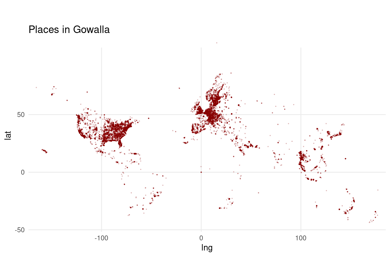
Places are mostly in the US, Europe, and Asia. Let’s keep only the ones in continental US
us_states <- states(cb = TRUE,progress=F) |> st_transform(crs = 4326)
continental_us <- us_states |>
filter(!STUSPS %in% c("AK", "HI", "AS", "GU", "MP", "PR", "VI"))Gowalla check-ins in the US
For simplicity, let’s keep only the check-ins, places, users, and social connections in the continental US. First, we get the points within the continental US
places_sf <- places |> st_as_sf(coords = c("lng", "lat"), crs = 4326)
places_sf <- places_sf |> st_join(continental_us,
                              join=st_within,
                              left=FALSE)
We have 1114850 places in the continental US. Let’s plot some of them
places_sf |> sample_n(30000) |>
  ggplot() + geom_sf(data = continental_us,fill="lightgray") +
  geom_sf(size=.01,color="darkred") + theme_minimal() +
  labs(title="Places in Gowalla in the continental US")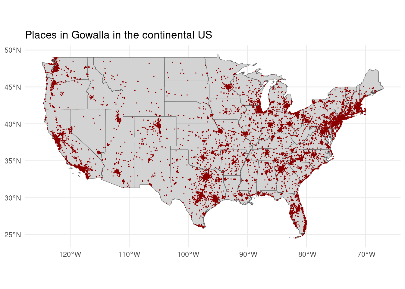
The categories in the continental US are a little bit different
places_sf |> st_drop_geometry() |>
  count(category) |> arrange(desc(n)) |> datatable()
Let’s keep only the check-ins in the continental US
checkins <- checkins |> filter(placeid %in% places_sf$id) We keep only relationships between users with check-ins in the continental US
users_us <- checkins |> select(userid) |> distinct() |> collect() |> pull(userid)
friendships <- friendships |>
  filter(userid1 %in% users_us & userid2 %in% users_us)
Relationship between social connections and mobility
Let’s use this dataset to see social connectivity and mobility relationships. Many processes are responsible for creating and maintaining social connections, including homophily, social influence, or geographical proximity [3]. Many articles have shown that geographical proximity and similarity are some of the most critical processes for social interactions [2].
Let’s see if this is true using the large-scale data from Gowalla. We will use the following approach:
- First, we will define the geographical proximity of users as the distance between the users’ home locations.
- Secondly, we will go beyond home distance and define the actual geographical similarity by computing the frequency of the places they co-visit.
- Finally, we will see if the geographical similarity is related to the probability of social connections between users.
Detecting homes
We don’t have the users’ home locations in our Gowalla dataset. However, we can use the users’ most visited places as a proxy for their home locations. Let’s compute the most visited places for the users. Because of the sparseness of the data, we will use H3 spatial index hexagons to aggregate the checkins. See appendix #sec-h3 for more information about the H3 spatial index.
places_sf <- places_sf |> mutate(h3 = point_to_cell(geometry, 7))Let’s add that information to the check-ins and assign each user’s most visited H3 hexagon as home location.
users_home <- checkins |>
  mutate(placeid=as.integer(placeid)) |>
  left_join(places_sf |> select(id,h3) |> st_drop_geometry(),
            join_by("placeid"=="id")) |>
  count(userid,h3) |> collect() |>
  group_by(userid) |> filter(n == max(n)) |>
  slice_head(n = 1)
Exercise
- Calculate the bias in the Gowalla dataset by investigating the relationship between the homes detected and the actual population.
- How can we calculate the population by H3 hexagon? One way is to use areal interpolation, which is a method to estimate an area’s population based on the surrounding areas’ population. We can use the WorldPop dataset or small census areas from ACS.
Exercise
- Calculate the distance people travel from home to check-in at different categories.
- Do you see any difference in the distance traveled to gas stations or restaurants?
Home distance between friends
Let’s investigate how far friends live in Gowalla. First, we add the lat and lon for each h3 centroid
coords <- cell_to_point(users_home$h3) |> st_coordinates()
users_home <- users_home |>
  ungroup() |>
  mutate(lat=coords[,2],lon=coords[,1])
Add the home location to the friendships.
friendships <- friendships |>
  left_join(users_home, by = c("userid1" = "userid")) |>
  rename(home1 = h3) |>
  left_join(users_home, by = c("userid2" = "userid")) |>
  rename(home2 = h3)
And calculate the distance between the homes. First we define a distance function
dist_cities_haver <- function(lon1,lat1,lon2,lat2){
  #calculates distances between points in km
  long1 <- lon1*pi/180; lat1 <- lat1*pi/180
  long2 <- lon2*pi/180; lat2 <- lat2*pi/180
  R <- 6371 # Earth mean radius [km]
  delta.long <- (long2 - long1); delta.lat <- (lat2 - lat1)
  a <- sin(delta.lat/2)^2 + cos(lat1) * cos(lat2) * sin(delta.long/2)^2
  c <- 2 * asin(ifelse(sqrt(a)<1,sqrt(a),1))
  R * c
}
friendships <- friendships |>
  mutate(distance = dist_cities_haver(lon.x,lat.x,lon.y,lat.y))
Let’s compare it with users which are not friends
users_all <- checkins |> select(userid) |>
  distinct() |> collect() |> pull()
no_friendships <-
  tibble(userid1=sample(users_all,1000000,replace=T),
         userid2=sample(users_all,1000000,replace=T))
no_friendships <- no_friendships |>
  left_join(users_home, by = c("userid1" = "userid")) |>
  rename(home1 = h3) |>
  left_join(users_home, by = c("userid2" = "userid")) |>
  rename(home2 = h3) |>
  mutate(distance = dist_cities_haver(lon.x,lat.x,lon.y,lat.y))
Here is the density to have a friend as a function of the distance between the homes
ggplot() +
  geom_density(data=friendships |> filter(n.x>=100 & n.y >= 100),
               aes(x=distance,col="Friends")) +
  geom_density(data=no_friendships |> filter(n.x>=100 & n.y >= 100),
               aes(x=distance,col="no Friends"))+
  labs(title="Density of friendships as a function of distance between homes")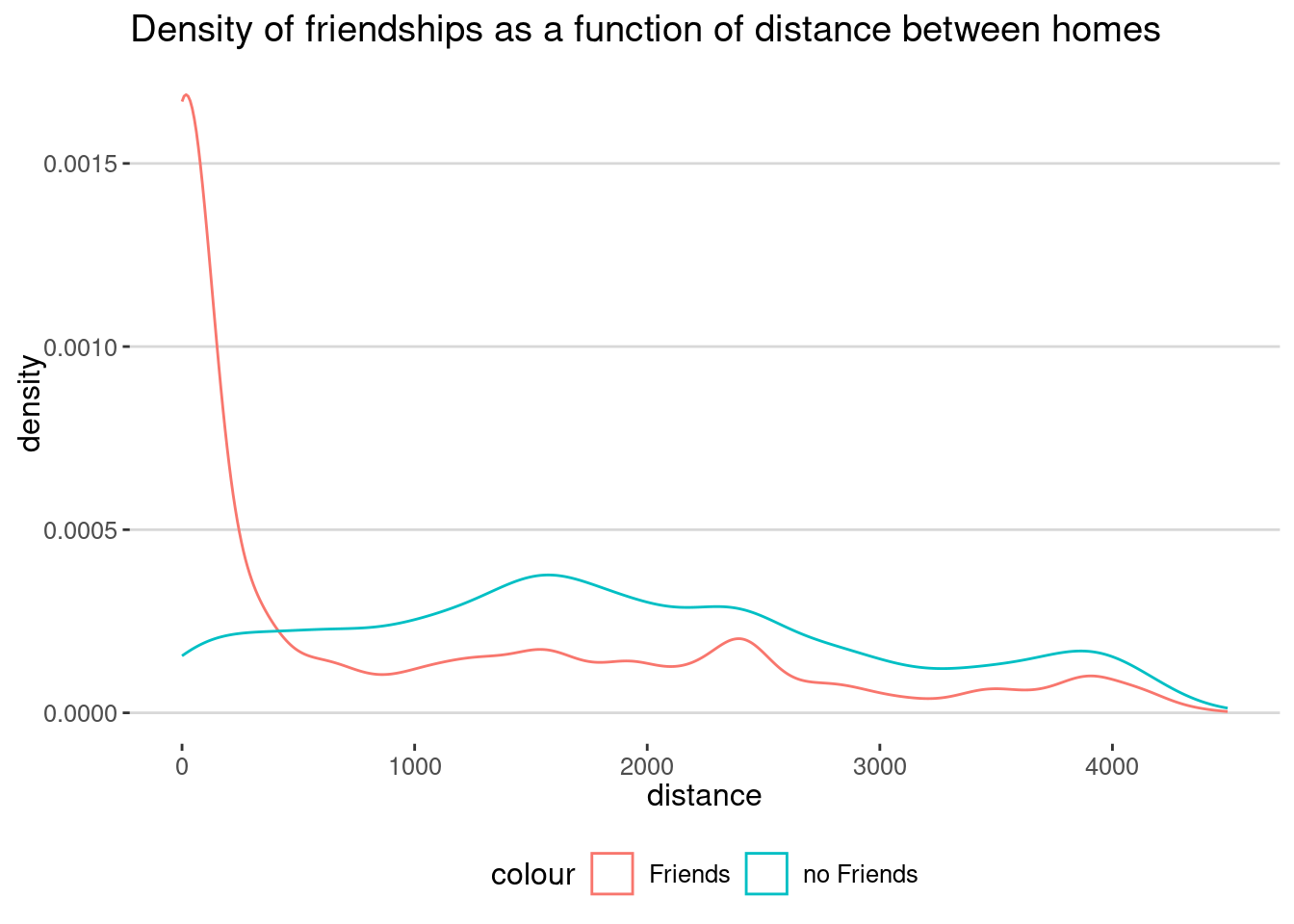
As we can see the majority of the friends live close to each other.
median(friendships$distance,na.rm = T)[1] 357.1501median(no_friendships$distance,na.rm = T)[1] 1745.38Mobility similarity
Our previous result shows that friends live close to each other. However, this is not enough to say that geographical proximity is the primary driver of social connections. We need to go beyond home distance and define the actual geographical similarity by computing the similarity of places they visit.
Let’s calculate the similarity of places visited by users. We will use the Jaccard similarity, which measures the similarity between two sets. The Jaccard similarity is defined as the size of the intersection divided by the size of the union of the two sets.
\[ J_{ij} = \frac{|A_i \cap A_j|}{|A_i \cup A_j|} \] where \(A_i\) and \(A_j\) are the sets of places visited by users \(i\) and \(j\).
As places, we are going to take the h3 hexagon where the check-ins are made:
checkins <- checkins |>
  mutate(placeid=as.integer(placeid)) |>
  left_join(places_sf |> select(id,h3) |> st_drop_geometry(),
            join_by("placeid"=="id")) |>
  rename(h3 = h3)
Let’s select a collection of users who are friends and a collection of users who are not friends
relationships_sel <-
  friendships |> sample_n(2000) |>
          select(userid1,userid2) |> mutate(friends=1) |>
  rbind(no_friendships |> sample_n(2000) |>
          select(userid1,userid2) |> mutate(friends=0)
  ) |>
  mutate(jaccard=0)
Select the check-ins of the users selected
users_sel_jaccard <- relationships_sel |>
  select(userid1,userid2) |>
  distinct() |>
  unlist() |> unique()

checkins_sel <- checkins |>
  mutate(userid=as.integer(userid)) |>
  filter(userid %in% users_sel_jaccard) |> collect() |>
  select(userid,h3) |>
  distinct()
Calculate the Jaccard similarity between users
relationships_sel <- relationships_sel |>
  mutate(jaccard=map2_dbl(userid1,userid2,~{
    h3_1 <- checkins_sel |> filter(userid == .x) |> pull(h3)
    h3_2 <- checkins_sel |> filter(userid == .y) |> pull(h3)
    length(intersect(h3_1,h3_2))/length(union(h3_1,h3_2))
  }))
Finally, let’s check how the probability of friendship depends on the Jaccard mobility similarity.
relationships_sel |>
  mutate(jaccard_bin = cut(jaccard,breaks = seq(0,1,.05))) |>
  group_by(jaccard_bin) |>
  summarise(friends = mean(friends),jaccard=median(jaccard),total = n()) |>
  ggplot(aes(x=jaccard,y=friends)) + geom_point() +
  scale_x_sqrt(limits=c(0,1)) +
  labs(title="Probability of friendships as a function of Jaccard similarity")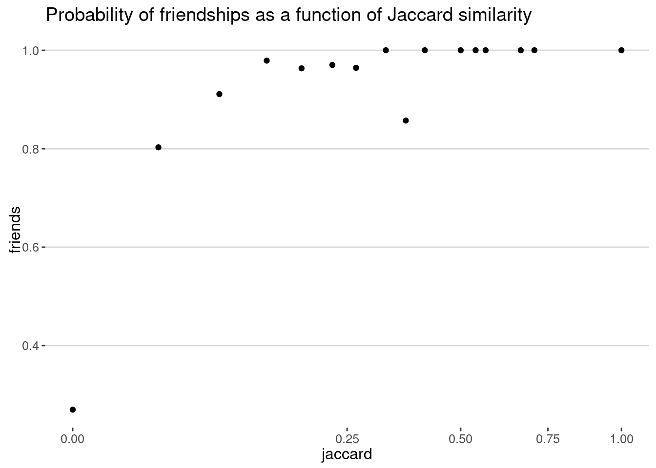
As we can see, the probability of friendship increases with the Jaccard similarity, a result found in many different papers (e.g., [2]).
Exercise
- How do the results depend on other resolutions?
- Although sparser, how could the results depend on whether we compute the similarity using the actual places visited, not the H3 hexagons?
- What if we use only some categories of places?
Conclusions
In this practical, we have used Location-Based Social Networks (the Gowalla dataset) to understand the relationship between social connections and mobility. We have seen that friends live close to each other and that the probability of friendship increases with the Jaccard similarity of places visited. This result is consistent with previous research that shows that geographical proximity and similarity are important drivers of social connections.
This strong relationship between social connections and mobility has important implications for urban science research. It suggests that social connections and mobility are closely related and that understanding one can help us understand the other. This relationship can be used to design better urban planning strategies, improve social recommendation algorithms, and understand human behavior in urban areas.
Appendix: H3 global grid system
H3 is a geospatial indexing system that divides the Earth’s surface into hexagons. It is a hierarchical system, meaning that each hexagon can be divided into smaller hexagons. H3 is useful for many geospatial applications, including spatial indexing, spatial aggregation, and spatial analysis.
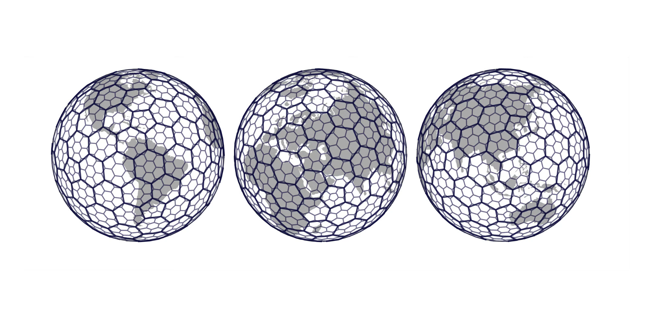
Geographical coordinates can be mapped to H3 hexagons, making it easier to work at aggregated levels to reduce the computational complexity of spatial operations. H3 is also useful for spatial indexing, as it allows for fast spatial queries and operations.
In R there are many packages to work with h3, including h3jsr which is a wrapper of the h3 library in JavaScript. Here is an example of how to use h3jsr to convert geographical coordinates to H3 hexagons:
require(h3jsr)
point_to_cell(c(40.7128, -74.0060), 5)
[1] "85f05ab7fffffff"and here is how to get the geographical coordinates (centroid) of an H3 hexagon:
cell_to_point("85489e37fffffff")Geometry set for 1 feature
Geometry type: POINT
Dimension: XY
Bounding box: xmin: -97.76681 ymin: 30.27655 xmax: -97.76681 ymax: 30.27655
Geodetic CRS: WGS 84H3 hexagons come in different resolutions, from 0 to 15. The resolution determines the size of the hexagons, with higher resolutions resulting in smaller hexagons. The resolution can be set when converting geographical coordinates to H3 hexagons:
point_to_cell(c(40.7128, -74.0060), 5)[1] "85f05ab7fffffff"cell_to_point("85f05ab7fffffff")Geometry set for 1 feature
Geometry type: POINT
Dimension: XY
Bounding box: xmin: 40.85487 ymin: -73.97816 xmax: 40.85487 ymax: -73.97816
Geodetic CRS: WGS 84here is the list of resolutions and the size of the hexagons in meters:
data("h3_info_table")
h3_info_table |> select(h3_resolution,avg_area_sqkm) |>
mutate(avg_area_sqkm = sprintf("%.8g",avg_area_sqkm)) |> kable()| h3_resolution | avg_area_sqkm |
|---|---|
| 0 | 4357449.4 |
| 1 | 609788.44 |
| 2 | 86801.78 |
| 3 | 12393.435 |
| 4 | 1770.3477 |
| 5 | 252.90386 |
| 6 | 36.129062 |
| 7 | 5.1612934 |
| 8 | 0.7373276 |
| 9 | 0.10533251 |
| 10 | 0.015047502 |
| 11 | 0.0021496431 |
| 12 | 0.00030709188 |
| 13 | 4.3870268e-05 |
| 14 | 6.2671811e-06 |
| 15 | 8.9531159e-07 |
References
[1]
D. Yang, B. Qu, J. Yang, and P. Cudre-Mauroux, “Revisiting User Mobility and Social Relationships in LBSNs: A Hypergraph Embedding Approach,” in The World Wide Web Conference, in WWW ’19. New York, NY, USA: Association for Computing Machinery, May 2019, pp. 2147–2157. doi: 10.1145/3308558.3313635.
[2]
E. Cho, S. A. Myers, and J. Leskovec, “Friendship and mobility: User movement in location-based social networks,” in Proceedings of the 17th ACM SIGKDD international conference on Knowledge discovery and data mining, in KDD ’11. New York, NY, USA: Association for Computing Machinery, Aug. 2011, pp. 1082–1090. doi: 10.1145/2020408.2020579.
[3]
M. L. Small and L. Adler, “The Role of Space in the Formation of Social Ties,” Annual Review of Sociology, vol. 45, no. Volume 45, 2019, pp. 111–132, Jul. 2019, doi: 10.1146/annurev-soc-073018-022707.
Social interactions
Finally, let’s load the social interactions between users. We have the reciprocal relationships between users:
Let’s see the distribution of the number of friends per user
As expected, it is a heavy-tailed distribution.