library(tidyverse)
library(arrow)
options(arrow.unsafe_metadata = TRUE)
library(DT) # for interactive tables
library(knitr) # for tables
library(ggthemes) # for ggplot themes
library(sf) # for spatial data
library(tigris) # for US geospatial data
library(tidycensus) # for US census data
library(fixest) #
theme_set(theme_hc() + theme(axis.title.y = element_text(angle = 90))) Lab 4-2 - Social media data
Geographical social networks
Objective
In this practical, we will use social media data to understand the interplay between geography, demography, and social interactions. We will focus on analyzing social media data from Foursquare about social connectivity between different areas in the US.
Specifically, we will:
- Understand the structure and nature of geographical social networks.
- Explore the data and understand the social connectivity within and across urban areas.
- Study the main determinants for social connectivity as a function of distance and demographic factors.
Load some libraries and settings we will use
Geographical Social Networks
Social media platforms allow us to collect information about where people live, how they move, and how they interact with each other. This information can be used to build geographical social networks, where nodes represent users or geographical areas (e.g., zip codes, census blocks) and edges represent social interactions between them [1].
Social Networks are impacted by geography. People tend to interact more with others who are geographically close to them [2] [3]. This is known as the proximity principle, a fundamental concept in urban sociology. It happens even in online social networks and online worlds [4], where physical distance is not a limitation [5].
On the other hand, since social networks are based on social interactions, they are also influenced by the social structure of cities and regions and the mobility of people in them.
Load the data
We will use the data at the county level in the US, which is already in the /data/CUS/Facebook_SCI/county/ folder. Let’s load the data and see what it looks like.
sci <- open_tsv_dataset("/data/CUS/FB_SCI/county_county.tsv.gz",
                           schema = schema(
                             user_loc = utf8(),
                             fr_loc = utf8(),
                             scaled_sci = int64()
                           ), skip = 1)
Let’s see the first rows of the data.
sci |> head() |> collect() |> kable()| user_loc | fr_loc | scaled_sci |
|---|---|---|
| 01001 | 01001 | 8946863 |
| 01001 | 01003 | 101997 |
| 01001 | 01005 | 134341 |
| 01001 | 01007 | 254620 |
| 01001 | 01009 | 67196 |
| 01001 | 01011 | 429022 |
Remember that each county in the US has a 5-digit GEOID. The first two digits of the GEOID represent the state, and the last three digits represent the county. For example, the GEOID for New York County is 36061 (36 is the state code for New York and 061 is the county code for New York County).
Preprocessing the data
This is the distribution of values of \(SCI_{ij}\)
sci %>% ggplot(aes(x=scaled_sci)) + geom_density() + scale_x_log10()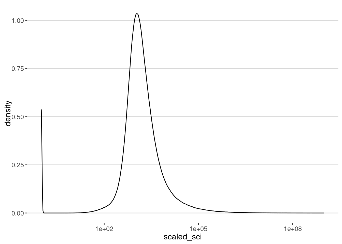
As we can see, there is an anomaly for very small numbers. SCI is scaled within each dataset to a maximum value of 1,000,000,000 and a minimum value of 1 (see the documentation of how SCI is built). This is why we have that anomaly at small values. Note that the actual value of SCI is not absolute since it is normalized for each dataset.
Let’s get rid of the anomaly of lower values. And also only keep different counties:
sci <- sci |> filter(scaled_sci >= 10)Impact of geographical distance on social connectivity
We first investigate how the SCI depends on the geographical distance between counties. We will use the geographical distance between the centroids of the counties as a proxy for the geographical distance between them. Let’s get the counties together with their median income, the fraction of people under the poverty line, and the total population.
cnts <- get_acs(geography = "county",
                variables = c(medincome = "B19013_001",
                              total_pob = "B01001_001",
                              poverty = "C17002_002"),
                output = "wide", year = 2019,
                geometry = T,cache_table = T,
                progress = F) |>
  mutate(povertyE = povertyE / total_pobE)
Let’s build a table that contains the information we want from that table, including the lat,lon of the centroid of the counties
tabla_counties <-
  tibble(GEOID=cnts$GEOID,
         pop=cnts$total_pobE,
         inc=cnts$medincomeE,
         pov=cnts$povertyE,
         st_coordinates(st_centroid(cnts$geometry)) |> as_tibble() %>%
           rename(lon=X,lat=Y))
And add that information to the \(SCI_{ij}\) table for the counties of the users and their friends
sci_expanded <- sci |>
  inner_join(tabla_counties, by = c("user_loc" = "GEOID")) |>
  rename(user_pop=pop,user_inc=inc,
         user_pov=pov,
         user_lat=lat,user_lon=lon) |>
  inner_join(tabla_counties, by = c("fr_loc" = "GEOID")) |>
  rename(fr_pop=pop,fr_inc=inc,
         fr_pov=pov,
         fr_lat=lat,fr_lon=lon)
sci_expanded |> head() |> collect() |> kable()| user_loc | fr_loc | scaled_sci | user_pop | user_inc | user_pov | user_lon | user_lat | fr_pop | fr_inc | fr_pov | fr_lon | fr_lat |
|---|---|---|---|---|---|---|---|---|---|---|---|---|
| 01001 | 01001 | 8946863 | 55380 | 58731 | 0.0620982 | -86.64274 | 32.5349 | 55380 | 58731 | 0.0620982 | -86.64274 | 32.53490 |
| 01001 | 01003 | 101997 | 55380 | 58731 | 0.0620982 | -86.64274 | 32.5349 | 212830 | 58320 | 0.0398581 | -87.72230 | 30.72677 |
| 01001 | 01005 | 134341 | 55380 | 58731 | 0.0620982 | -86.64274 | 32.5349 | 25361 | 32525 | 0.1329601 | -85.39343 | 31.86950 |
| 01001 | 01007 | 254620 | 55380 | 58731 | 0.0620982 | -86.64274 | 32.5349 | 22493 | 47542 | 0.0797137 | -87.12650 | 32.99858 |
| 01001 | 01009 | 67196 | 55380 | 58731 | 0.0620982 | -86.64274 | 32.5349 | 57681 | 49358 | 0.0645967 | -86.56755 | 33.98080 |
| 01001 | 01011 | 429022 | 55380 | 58731 | 0.0620982 | -86.64274 | 32.5349 | 10248 | 37785 | 0.1332943 | -85.71565 | 32.10053 |
For simplicity, let’s keep only the SCI within the continental US
sci_expanded <- sci_expanded |>
  filter(!substr(user_loc,1,2) %in% c("02","15","60","72","78")) |>
  filter(!substr(fr_loc,1,2) %in% c("02","15","60","72","78"))
Let’s have a look at the geographical distribution of friends for a particular county. Here is the SCI for the Suffolk county in MA
sci_suffolk <- sci_expanded |> filter(user_loc == "25025") |> collect()
cnts |> inner_join(sci_suffolk, by = c("GEOID" = "fr_loc")) |>
  ggplot(aes(fill=scaled_sci)) + geom_sf(col=rgb(0,0,0,0)) + theme_minimal() +
  scale_fill_viridis_c(trans="log") + labs(title="SCI for Suffolk County")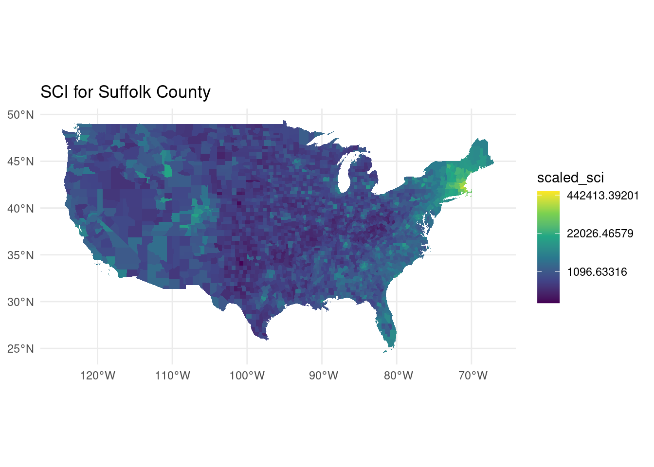
And here is for the Los Angeles County in CA
sci_la <- sci_expanded |> filter(user_loc == "06037") |> collect()
cnts |> inner_join(sci_la, by = c("GEOID" = "fr_loc")) |>
  ggplot(aes(fill=scaled_sci)) + geom_sf(col=rgb(0,0,0,0)) + theme_minimal() +
  scale_fill_viridis_c(trans="log") + labs(title="SCI for LA County")
Finally, here is the distribution for one of the poorest counties in the US, the Claiborne County in Mississippi
sci_clairborne <- sci_expanded |> filter(user_loc == "28021") |> collect()
cnts |> inner_join(sci_clairborne, by = c("GEOID" = "fr_loc")) |>
  ggplot(aes(fill=scaled_sci)) + geom_sf(col=rgb(0,0,0,0)) + theme_minimal() +
  scale_fill_viridis_c(trans="log") + labs(title="SCI for Claiborne County")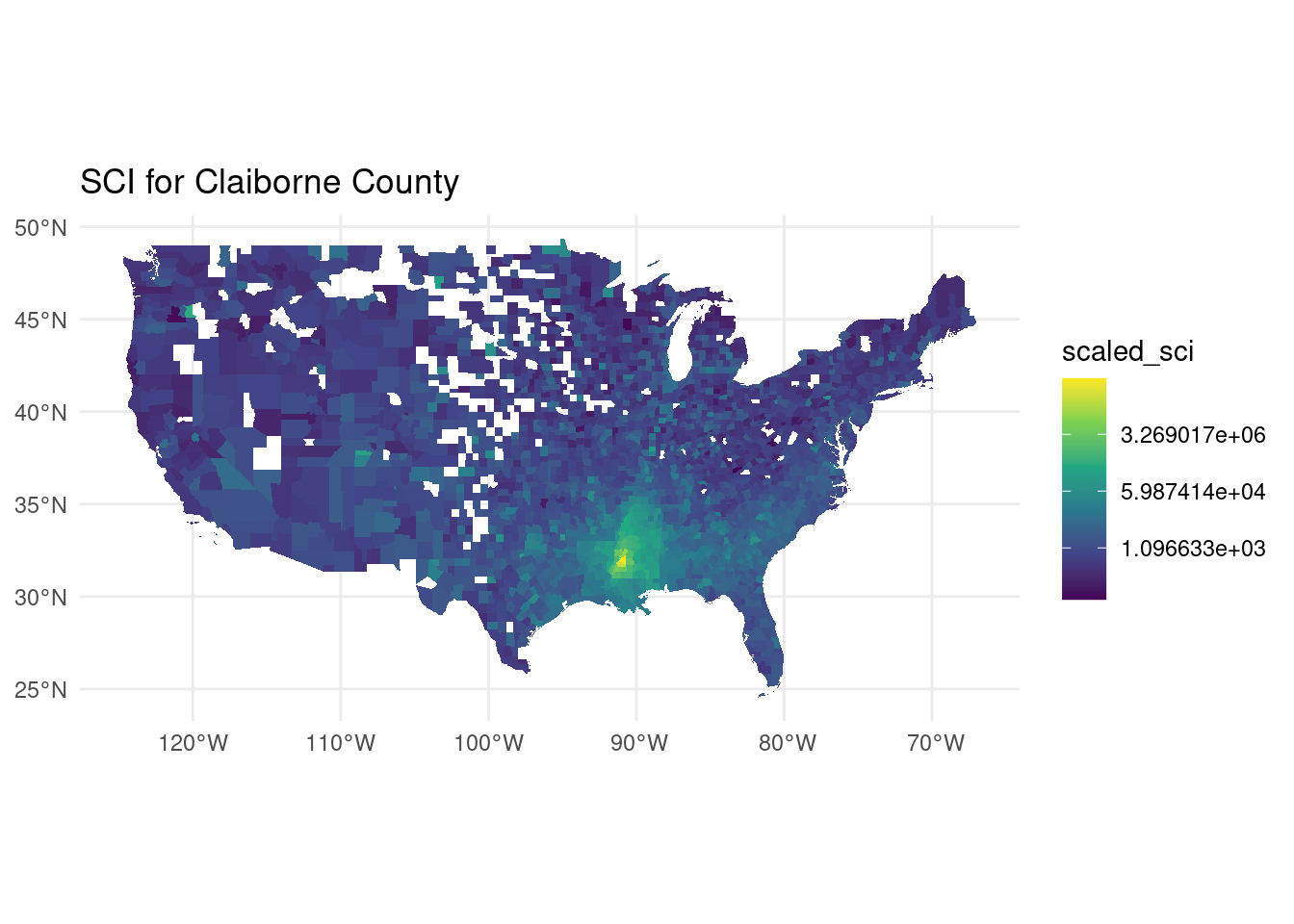
As we can see, most of the friends are in the counties around the county of interest. We also note that in the US, there are a lot of friendships across the country for high-income areas, while for low-income areas, the friendships are mostly local.
Distance between counties
We can then calculate the distance between counties using the Haversine formula. We only keep different counties
dist_cities_haver <- function(lon1,lat1,lon2,lat2){
  #calculates distances between points in km
  long1 <- lon1*pi/180; lat1 <- lat1*pi/180
  long2 <- lon2*pi/180; lat2 <- lat2*pi/180
  R <- 6371 # Earth mean radius [km]
  delta.long <- (long2 - long1); delta.lat <- (lat2 - lat1)
  a <- sin(delta.lat/2)^2 + cos(lat1) * cos(lat2) * sin(delta.long/2)^2
  c <- 2 * asin(ifelse(sqrt(a)<1,sqrt(a),1))
  R * c
}
sci_expanded <- sci_expanded |> collect() |>
  filter(user_loc != fr_loc) |>
  mutate(dist=dist_cities_haver(user_lon,user_lat,fr_lon,fr_lat))
How does \(SCI_{ij}\) depend on \(d_{ij}\)? (Note the logarithmic scale in the legend)
ggplot(sci_expanded,aes(x=dist,y=scaled_sci)) + geom_bin2d() +
  scale_fill_gradient(low="lightgray",high="black",trans="log10") +
  scale_x_log10() + scale_y_log10() + labs(x="d_ij",y="SCI_ij") +
  labs(x="Distance (km)",y="SCI (scaled)") + theme_minimal()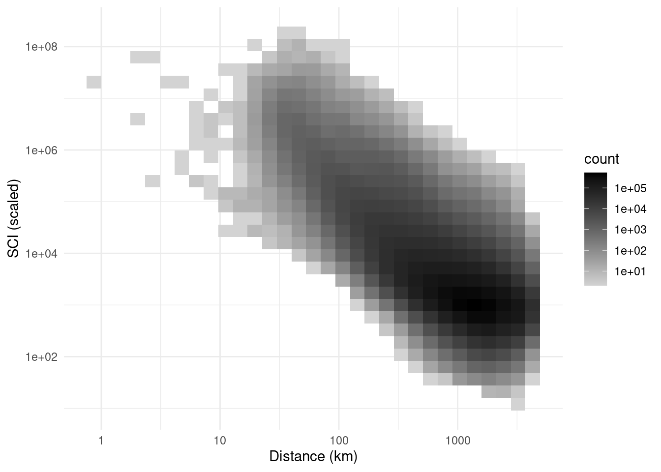
The correlation is very large (in logs)
cor.test(log(sci_expanded$scaled_sci),log(sci_expanded$dist),use="na")
    Pearson's product-moment correlation

data:  log(sci_expanded$scaled_sci) and log(sci_expanded$dist)
t = -2689, df = 9487372, p-value < 2.2e-16
alternative hypothesis: true correlation is not equal to 0
95 percent confidence interval:
 -0.6580084 -0.6572861
sample estimates:
       cor
-0.6576474 Geographical mesostructure of social networks
Although geographical distance is a strong predictor of social connectivity and being in the same state increases the probability of friendship, our social networks are not only determined by geographical distance or administrative borders. What are the typical areas in which social interactions happen? Are they cities, neighborhoods, or regions?
To answer this question, we can use the Louvain algorithm to detect communities in the geographical social network. The Louvain algorithm is a community detection algorithm that optimizes the network’s modularity. It is a fast and scalable algorithm that can detect communities in large networks.
Let’s build a geographical social network using the \(SCI_{ij}\) data. We will use the igraph package to build the network. Since \(SCI_{ij}\) is very big we are going to keep only the large values of ti
sci_pruned <- sci_expanded |> filter(scaled_sci > 1000) |> collect()Let’s form the graph
library(igraph)
g <- graph_from_data_frame(sci_pruned,directed=F)
g
IGRAPH 6f4bf25 UN-- 3108 6264684 --
+ attr: name (v/c), scaled_sci (e/n), user_pop (e/n), user_inc (e/n),
| user_pov (e/n), user_lon (e/n), user_lat (e/n), fr_pop (e/n), fr_inc
| (e/n), fr_pov (e/n), fr_lon (e/n), fr_lat (e/n), dist (e/n)
+ edges from 6f4bf25 (vertex names):
[1] 01001--01003 01001--01005 01001--01007 01001--01009 01001--01011
[6] 01001--01013 01001--01015 01001--01017 01001--01019 01001--01021
[11] 01001--01023 01001--01025 01001--01027 01001--01029 01001--01031
[16] 01001--01033 01001--01035 01001--01037 01001--01039 01001--01041
[21] 01001--01043 01001--01045 01001--01047 01001--01049 01001--01051
[26] 01001--01053 01001--01055 01001--01057 01001--01059 01001--01061
+ ... omitted several edgesCalculate the communities using the \(SCI_{ij}\) as the weight of the edges
coms <- cluster_louvain(g,weights=E(g)$scaled_sci)We got 12 communities. Let’s see the distribution of the size of the communities
table(membership(coms)) |> as.data.frame() |>
  ggplot(aes(Freq)) + geom_histogram() + theme_minimal()+
  labs(title="Distribution of the size of the communities",x="Size of the community",y="Frequency")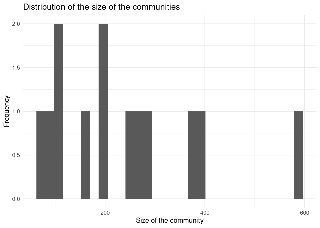
Create the table of communities
table_comm <- membership(coms) |> enframe(name="GEOID",value="comm")Merge with the original table of counties
cnts <- cnts |> inner_join(table_comm)Let’s visualize it
cnts |>
  filter(!substr(GEOID,1,2) %in% c("02","15","60","72","78")) |>
  ggplot(aes(fill=as.factor(comm))) + geom_sf(col=rgb(0,0,0,0)) +
  theme_minimal() + geom_sf(aes(fill=factor(comm)),col=rgb(0,0,0,0)) +
  scale_fill_tableau("Tableau 20") + theme_void()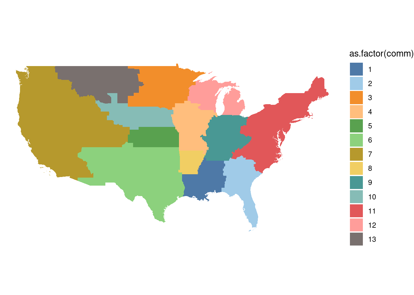
As we can see communities are geographically contiguous areas, an indication of the importance of distance in the Social Connectivity Index.
These communities are geographical areas where it is more likely to have friends within that across them. They are not necessarily administrative areas, but they are areas where most social interactions happen. Our results are very similar to other studies that have used different data sources to detect communities in social networks [1] [7].
Exercise
Use different community finding algorithms to detect communities in the geographical social network. Compare the results with the Louvain algorithm.
Repeat this exercise for the zip-zip level data for a particular state, city, or region. How do the communities change at this level? You can find the zip-level data in the
/data/CUS/FB_SCIfolder.
Conclusion
Social media data like the Facebook Social Connectivity Index can be used to understand geographical social networks. These networks are influenced by
- geographical distance,
- administrative borders, and
- demographics.
Social networks have different meso-structures than administrative areas. Community-finding algorithms can be used to detect those “functional” areas where most of our social interactions happen.
References
[1]
C. Herrera-Yagüe et al., “The anatomy of urban social networks and its implications in the searchability problem,” Scientific Reports, vol. 5, no. 1, p. 10265, Jun. 2015, doi: 10.1038/srep10265.
[2]
D. Liben-Nowell, J. Novak, R. Kumar, P. Raghavan, and A. Tomkins, “Geographic routing in social networks,” Proceedings of the National Academy of Sciences, vol. 102, no. 33, pp. 11623–11628, Aug. 2005, doi: 10.1073/pnas.0503018102.
[3]
J. Leskovec and E. Horvitz, “Geospatial Structure of a Planetary-Scale Social Network,” IEEE Transactions on Computational Social Systems, vol. 1, no. 3, pp. 156–163, Sep. 2014, doi: 10.1109/TCSS.2014.2377789.
[4]
M. Szell, R. Lambiotte, and S. Thurner, “Multirelational organization of large-scale social networks in an online world,” Proceedings of the National Academy of Sciences, vol. 107, no. 31, pp. 13636–13641, Aug. 2010, doi: 10.1073/pnas.1004008107.
[5]
B. Lengyel, A. Varga, B. Ságvári, Á. Jakobi, and J. Kertész, “Geographies of an Online Social Network,” PLOS ONE, vol. 10, no. 9, p. e0137248, Sep. 2015, doi: 10.1371/journal.pone.0137248.
[7]
F. Calabrese et al., “The Connected States of America: Quantifying Social Radii of Influence,” in 2011 IEEE Third International Conference on Privacy, Security, Risk and Trust and 2011 IEEE Third International Conference on Social Computing, Oct. 2011, pp. 223–230. doi: 10.1109/PASSAT/SocialCom.2011.247.
Social Media Data to understand geographical social networks
Most social networks generally have meta-data (or estimations) about where people live. That information is typically used for advertising purposes, but it can also be used to understand the social structure of cities and regions.
One particular example is Facebook, which publishes aggregate data about the social connections between different areas in the US. This data is based on the number of friendships between different pairs of areas, and it can be used to understand the social connectivity between different regions.