library(tidyverse)
library(DT) # for interactive tables
library(knitr) # for tables
library(ggthemes) # for ggplot themes
library(sf) # for spatial data
library(tigris) # for US geospatial data
library(tidycensus) # for US census data
library(stargazer) # for tables
library(leaflet) # for interactive maps
theme_set(theme_hc() + theme(axis.title.y = element_text(angle = 90))) Lab 8-2 - Population Mobility Models
Objectives
In this lab we will analyze the mobility of people in the US using aggregated mobility models. Specifically, we will:
- Use the flows between Counties and Census Tracts in the US from LBS data from Safegraph
- Use this data to estimate several models (gravity, radiation).
- Analyze the impact of the COVID-19 pandemic on mobility patterns.
Load some libraries and settings we will use
Load the data
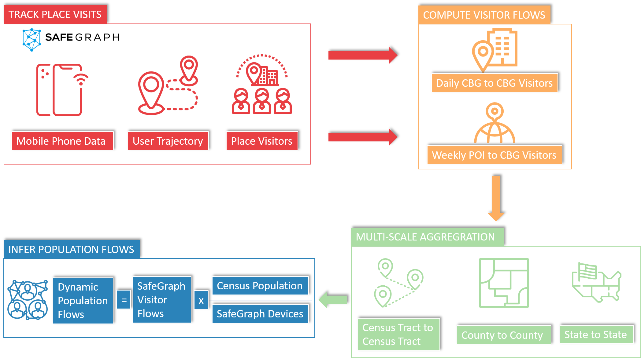
The data we will use was put together by the GeoDS Lab at the Department of Geography, University of Wisconsin-Madison. The data is published in Scientific Data [1] and is available at their github repository
The data is a matrix of weekly and monthly flows of individuals between counties and census tracts in the US. The authors used post-stratification techniques to account for the potential biases in the data.
The data is available in the following folders in stella
Weekly flows between states and counties from 2019 to 2021 in the
/data/CUS/COVID19USFlows-WeeklyFlowsfolder.Weekly flows between Census Tracts for 2019 in the
/data/CUS/COVID19USFlows-WeeklyFlows-Ct2019folder.
Let’s load the before and after the lockdowns by county for the week of March 2nd 2020, just before the lockdown, and for April 6th 2020, during the lockdown
flows_before <- read_csv("/data/CUS/COVID19USFlows-WeeklyFlows/weekly_flows/county2county/weekly_county2county_2020_03_02.csv")
flows_after <- read_csv("/data/CUS/COVID19USFlows-WeeklyFlows/weekly_flows/county2county/weekly_county2county_2020_04_06.csv")
flows_before |> head() |> datatable()
Note that the we have two columns for the flows:
visitor_flows: the number of visitors from the origin to the destination from the raw datapop_flows: the number of visitors from the origin to the destination after post-stratification
Let’s get the counties from tidycensus including their population
require(tidycensus)
counties <- get_acs(geography = "county",
                    variables = "B01003_001",year=2020,
                    geometry = TRUE,
                    progress = F)
Let’s see the flows. We keep only the continental US counties
no_continental <- c("02","15","60","66","69","72","78")
flows_before <- flows_before |>
  filter(!substr(geoid_o,1,2) %in% no_continental) |>
  filter(!substr(geoid_d,1,2) %in% no_continental)
flows_after <- flows_after |>
  filter(!substr(geoid_o,1,2) %in% no_continental) |>
  filter(!substr(geoid_d,1,2) %in% no_continental)
counties <- counties |>
  filter(!substr(GEOID,1,2) %in% no_continental)
Here is the mobility before the lockdown:
flows_before |> filter(pop_flows > 8000) |>
  ggplot() +
  geom_sf(data=counties,col="grey",fill="white",alpha=0.5,size=0.01) +
  geom_segment(aes(x=lng_o,y=lat_o,xend=lng_d,yend=lat_d,
                   alpha=log(pop_flows)),size=.5,col="darkgreen") +
  theme_void() + labs(title = "Mobility Flows, March 2nd 2020")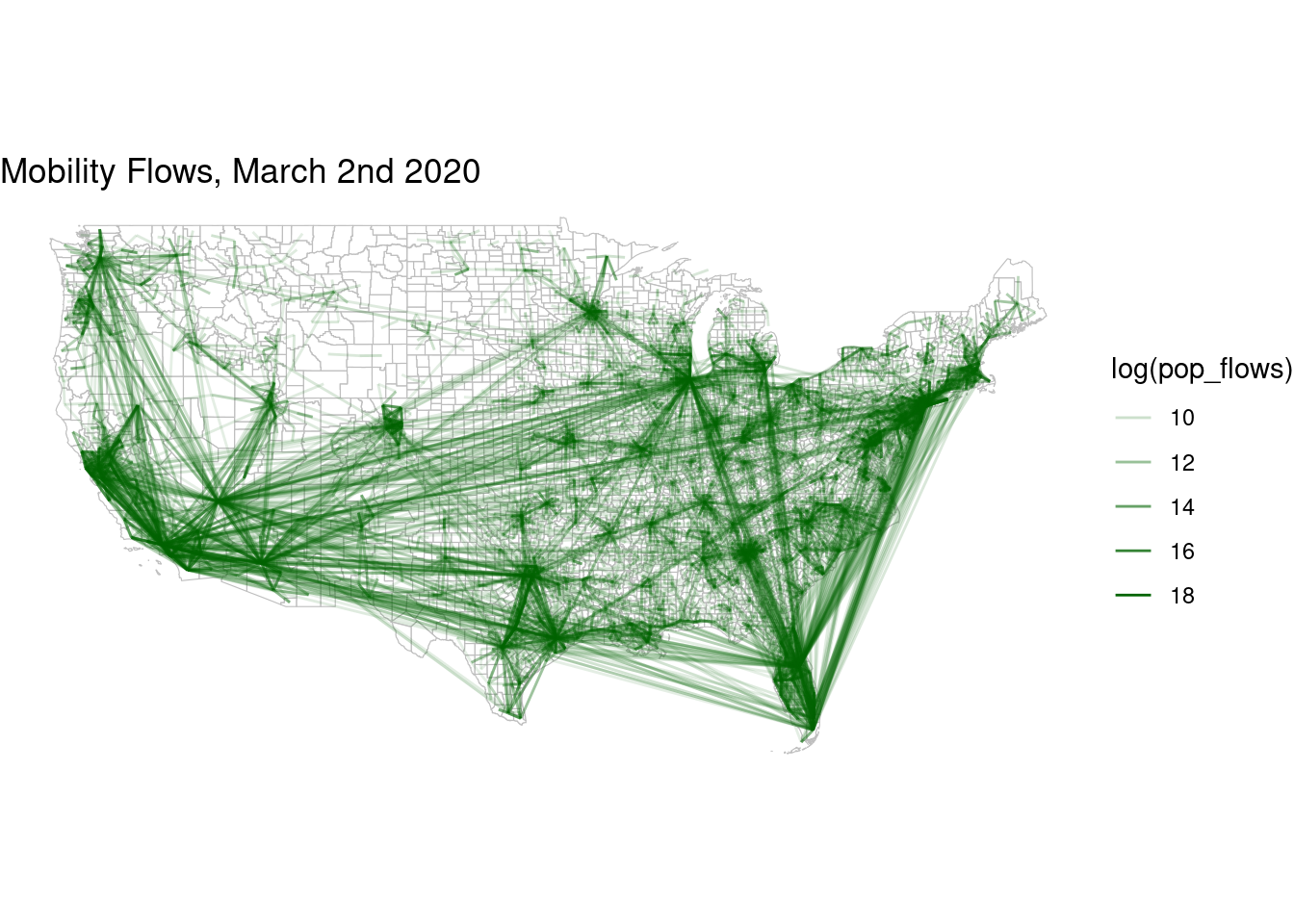
and after
flows_after |> filter(pop_flows > 8000) |>
  ggplot() +
  geom_sf(data=counties,col="grey",fill="white",alpha=0.5,size=0.01) +
  geom_segment(aes(x=lng_o,y=lat_o,xend=lng_d,yend=lat_d,
                   alpha=log(pop_flows)),size=.5,col="darkgreen") +
  theme_void() + labs(title = "Mobility Flows, April 6th 2020")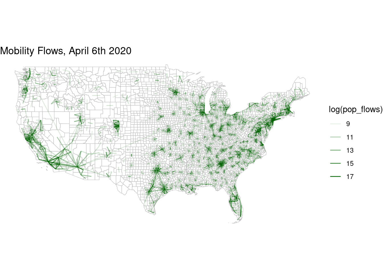
Gravity models
We will use the gravity model to estimate the flows between counties. The gravity model is a simple model that assumes that the flow between two locations is proportional to the product of their populations and inversely proportional to the distance between them. The model is given by:
\[ T_{ij} \sim \frac{P_i P_j}{d_{ij}^\beta} \]
where \(T_{ij}\) is the flow between locations \(i\) and \(j\), \(P_i\) and \(P_j\) are the populations of locations \(i\) and \(j\), \(d_{ij}\) is the distance between locations \(i\) and \(j\), and \(\gamma\) is a parameter that determines the strength of the distance effect.
First we prepare the data to estimate the model. We will use the flows from the week before the lockdown
flows_before <- flows_before |>
  left_join(counties |> st_drop_geometry(),
            by=c("geoid_o"="GEOID")) |>
  rename(pop_o = estimate) |>
  left_join(counties |> st_drop_geometry(),
            by=c("geoid_d"="GEOID")) |>
  rename(pop_d = estimate)
Let’s also include the distance between the counties:
dist_cities_haver <- function(lon1,lat1,lon2,lat2){
  # lo primero que hay que hacer es convertir todo a radianes
  long1 <- lon1*pi/180
  lat1 <- lat1*pi/180
  long2 <- lon2*pi/180
  lat2 <- lat2*pi/180
  R <- 6371 # Earth mean radius [km]
  delta.long <- (long2 - long1)
  delta.lat <- (lat2 - lat1)
  a <- sin(delta.lat/2)^2 + cos(lat1) * cos(lat2) * sin(delta.long/2)^2
  c <- 2 * asin(ifelse(sqrt(a)<1,sqrt(a),1))
  d = R * c
  return(d)
}
flows_before <- flows_before |>
  mutate(dist = dist_cities_haver(lng_o,lat_o,lng_d,lat_d))
Here is the data for the model
data_model <- flows_before |>
  filter(dist > 0)
There are several ways to fit the gravity model.
Using non-linear regression
We can use non-linear regression to estimate the parameters of the gravity model. We will use the nls function in R to estimate the parameters of the model.
gravity_nls <- nls(pop_flows ~ k * pop_o * pop_d / (dist)^gamma,
                   data= data_model,
                   start=list(k = 0.001, gamma=1),
                   algorithm="port",
                   lower = list(gamma = 0),
                   upper = list(gamma = 10))
Let’s see the results
data_model |>
  mutate(pred = fitted(gravity_nls)) |>
  ggplot(aes(x=pop_flows,y=pred)) + geom_bin2d() +
  scale_x_log10() + scale_y_log10() +
  scale_fill_continuous(name="Count",
                        trans = "log",
                        low = "white", high = "darkblue",
                        breaks = scales::log_breaks(),  # Set log-based breaks
                        labels = scales::label_number() ) + # Convert labels back to real numbers
  labs(title="NLS Gravity model fit",x="Observed flows",y="Predicted flows")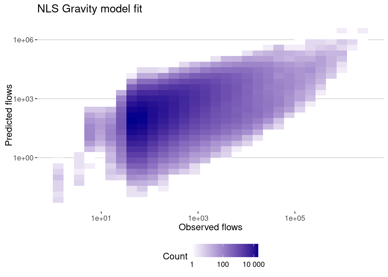
To quantify the error of the model we can use different metrics:
- The correlation between the real and predicted flows or coefficient \(R\)
- The correlation between the log of real and predicted flows.
- The most common metric used to evaluate the performance of flow generation models is the Common Part of Commuters (CPC) index:
\[ CPC = \frac{2 \sum_{ij} \text{min}(T_{it},\hat T_{ij})}{\sum_{ij} T_{ij} + \sum_{ij} \hat T_{ij}} \]
which we can implement in R:
cpc <- function(flow,hatflow){
  return(2*sum(pmin(flow,hatflow))/(sum(flow)+sum(hatflow)))
}
Let’s get the errors:
cor_gravity_nls <- flows_before |>
  filter(dist>0) |>
  mutate(pred = fitted(gravity_nls)) |>
  summarize(cor_values = cor(pop_flows,pred),
            cor_log_values=cor(log(pop_flows),log(pred)),
            cpc = cpc(pop_flows,pred))
cor_gravity_nls
# A tibble: 1 × 3
cor_values cor_log_values cpc
<dbl> <dbl> <dbl>
1 0.624 0.445 0.375Using linear regression
Because the gravity model is a non-linear model, it is often better to fit it in the log-space. This way the fitting is not affected by large values or outliers. We can use the lm function in R to estimate the parameters of the gravity model.
gravity_lm <-
  lm(log(pop_flows/(pop_o*pop_d)) ~ log(dist), data=data_model)
summary(gravity_lm)
Call:
lm(formula = log(pop_flows/(pop_o * pop_d)) ~ log(dist), data = data_model)

Residuals:
    Min      1Q  Median      3Q     Max
-6.6262 -1.2047 -0.1387  1.0656  9.3394

Coefficients:
             Estimate Std. Error t value Pr(>|t|)
(Intercept) -8.889544   0.013233  -671.8   <2e-16 ***
log(dist)   -1.477467   0.002085  -708.8   <2e-16 ***
---
Signif. codes:  0 '***' 0.001 '**' 0.01 '*' 0.05 '.' 0.1 ' ' 1

Residual standard error: 1.713 on 570105 degrees of freedom
Multiple R-squared:  0.4684,    Adjusted R-squared:  0.4684
F-statistic: 5.024e+05 on 1 and 570105 DF,  p-value: < 2.2e-16
Let’s see the results
data_model |>
  mutate(pred = exp(fitted(gravity_lm))*pop_o*pop_d) |>
  ggplot(aes(x=pop_flows,y=pred)) + geom_bin2d() +
  scale_x_log10() + scale_y_log10() +
  scale_fill_continuous(name="Count",
                        trans = "log",
                        low = "white", high = "darkblue",
                        breaks = scales::log_breaks(),  # Set log-based breaks
                        labels = scales::label_number() ) + # Convert labels back to real numbers
  labs(title="NLS Gravity model fit",x="Observed flows",y="Predicted flows")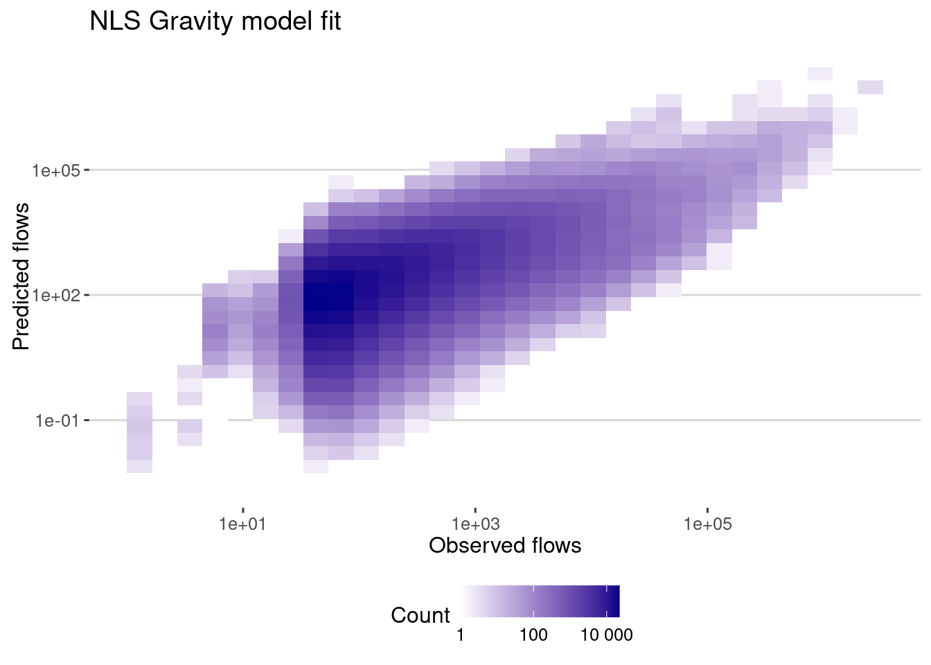
And here is the correlation
cor_gravity_lm <-
  flows_before |>
  filter(dist>0) |>
  mutate(pred = exp(fitted(gravity_lm))*pop_o*pop_d) |>
  summarize(cor_values = cor(pop_flows,pred),
            cor_log_values=cor(log(pop_flows),log(pred)),
            cpc = cpc(pop_flows,pred))
cor_gravity_lm
# A tibble: 1 × 3
cor_values cor_log_values cpc
<dbl> <dbl> <dbl>
1 0.477 0.552 0.428As expected, the correlation in log-values is higher when we fit the model in the log-space. Note also that the CPC is higher.
The gravity model used so far assumes that the number of flows originated from \(i\) is proportional to the population and the number of opportunities at \(j\) is proportional to \(P_j\). This is a simplification that might not be true. For example, the number of opportunities in \(j\) might scale like \(P_j^{\alpha_j}\). Thus, we can use a more general model that includes the population of the origin and the destination as exponents of the population. The model is given by:
\[ T_{ij} \sim \frac{P_i^{\alpha_i} P_j^{\alpha_j}}{d_{ij}^\beta} \]
We can estimate the parameters using the same approach as before.
gravity_lm_general <-
  lm(log(pop_flows) ~ log(pop_o) + log(pop_d) + log(dist), data=data_model)
Let’s see the results
data_model |>
  mutate(pred = exp(fitted(gravity_lm_general))) |>
  ggplot(aes(x=pop_flows,y=pred)) + geom_bin2d() +
  scale_x_log10() + scale_y_log10() +
  scale_fill_continuous(name="Count",
                        trans = "log",
                        low = "white", high = "darkblue",
                        breaks = scales::log_breaks(),  # Set log-based breaks
                        labels = scales::label_number() ) + # Convert labels back to real numbers
  labs(title="NLS Gravity model fit",x="Observed flows",y="Predicted flows")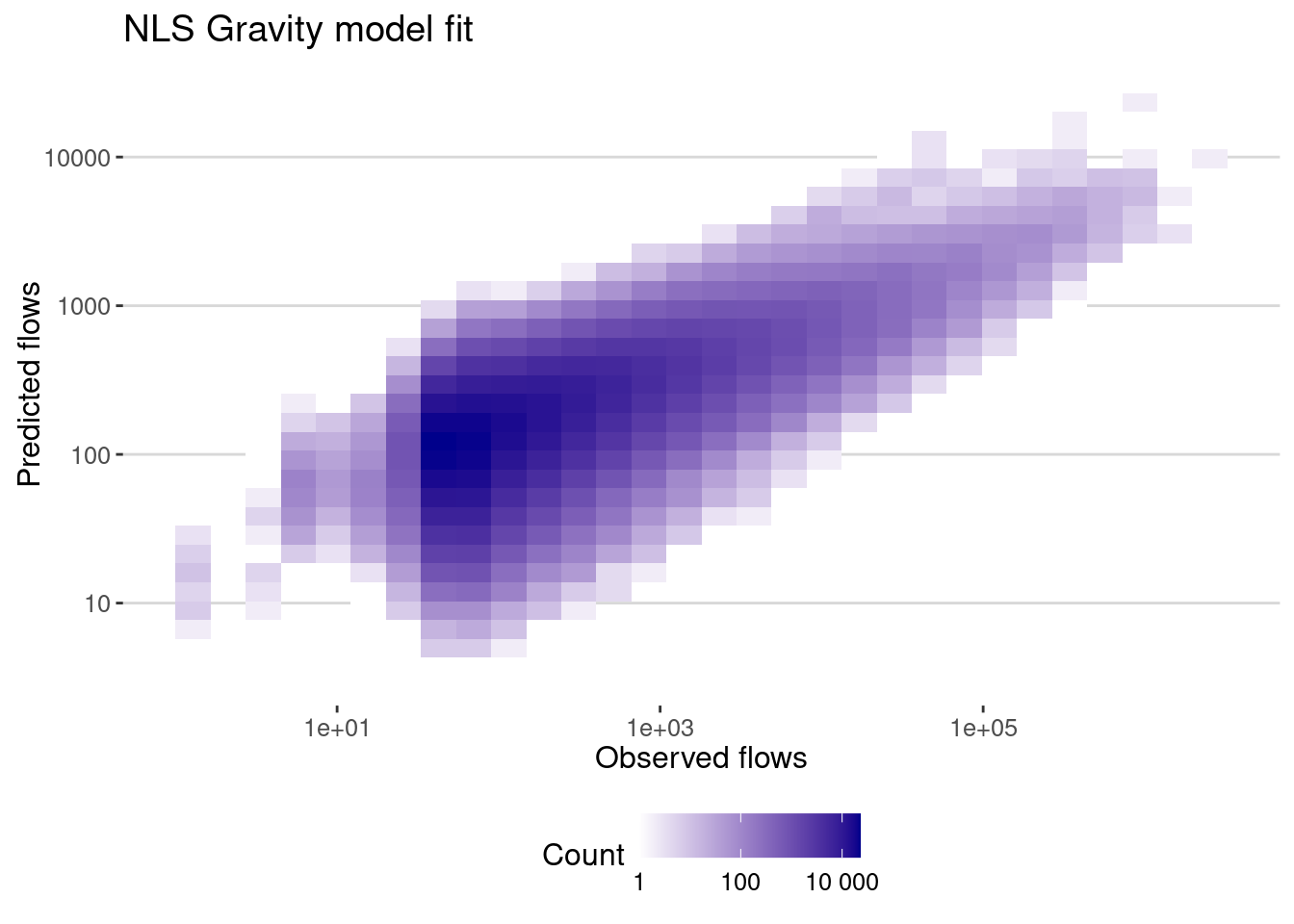
And here is the correlation
cor_gravity_lm_general <- flows_before |>
  filter(dist>0) |>
  mutate(pred = exp(fitted(gravity_lm_general))) |>
  summarize(cor_values = cor(pop_flows,pred),
            cor_log_values=cor(log(pop_flows),log(pred)),
            cpc = cpc(pop_flows,pred))
cor_gravity_lm_general
# A tibble: 1 × 3
cor_values cor_log_values cpc
<dbl> <dbl> <dbl>
1 0.539 0.609 0.229As we can see the correlation is higher when we using only the populations, but the CPC is smaller. Let’s compare the coefficients:
require(stargazer)
stargazer(gravity_lm,gravity_lm_general,type="html")| Dependent variable: | ||
| log(pop_flows/(pop_o * pop_d)) | log(pop_flows) | |
| (1) | (2) | |
| log(pop_o) | 0.273*** | |
| (0.001) | ||
| log(pop_d) | 0.371*** | |
| (0.001) | ||
| log(dist) | -1.477*** | -0.790*** |
| (0.002) | (0.001) | |
| Constant | -8.890*** | 2.493*** |
| (0.013) | (0.015) | |
| Observations | 570,107 | 570,107 |
| R2 | 0.468 | 0.371 |
| Adjusted R2 | 0.468 | 0.371 |
| Residual Std. Error | 1.713 (df = 570105) | 1.065 (df = 570103) |
| F Statistic | 502,373.500*** (df = 1; 570105) | 112,087.800*** (df = 3; 570103) |
| Note: | p<0.1; p<0.05; p<0.01 | |
As we can see, the exponents for the populations are smaller than one, which means that the number of flows is sublinear with the population of the origin and the destination. They are also different, which means that there is an asymmetry in the flows.
Using Poisson regression
Mobility flows are often modeled as count data and, thus, we should use a model that accounts for that. In general, gravity models are then fitted using Poisson regressions, in which the \(T_{ij}\) are Poissonian variables sampled with mean \(\lambda_{ij}\) which is model as
\[ \log(\lambda_{ij}) = \log(k) + \alpha \log(P_i) + \beta \log(P_j) - \gamma \log(d_{ij}) \]
where \(k\) is a constant, \(\alpha\) and \(\beta\) are the exponents of the populations, and \(\gamma\) is the exponent of the distance. We will use the glm function in R to estimate the parameters of the model.
gravity_glm_poisson <-
  glm(pop_flows ~ log(pop_o) + log(pop_d) + log(dist), data=data_model,family=poisson(link="log"))
Here is the error of the model
cor_gravity_glm_poisson <-
  data_model |>
  mutate(pred = fitted(gravity_glm_poisson)) |>
  summarize(cor_values = cor(pop_flows,pred),
            cor_log_values=cor(log(pop_flows),log(pred)),
            cpc = cpc(pop_flows,pred))
cor_gravity_glm_poisson
# A tibble: 1 × 3
cor_values cor_log_values cpc
<dbl> <dbl> <dbl>
1 0.483 0.606 0.520And the comparison between the models
stargazer(gravity_lm,gravity_lm_general,gravity_glm_poisson,type="html")| Dependent variable: | |||
| log(pop_flows/(pop_o * pop_d)) | log(pop_flows) | pop_flows | |
| OLS | OLS | Poisson | |
| (1) | (2) | (3) | |
| log(pop_o) | 0.273*** | 0.469*** | |
| (0.001) | (0.00003) | ||
| log(pop_d) | 0.371*** | 0.745*** | |
| (0.001) | (0.00003) | ||
| log(dist) | -1.477*** | -0.790*** | -1.642*** |
| (0.002) | (0.001) | (0.00003) | |
| Constant | -8.890*** | 2.493*** | 1.547*** |
| (0.013) | (0.015) | (0.0004) | |
| Observations | 570,107 | 570,107 | 570,107 |
| R2 | 0.468 | 0.371 | |
| Adjusted R2 | 0.468 | 0.371 | |
| Log Likelihood | -520,213,036.000 | ||
| Akaike Inf. Crit. | 1,040,426,081.000 | ||
| Residual Std. Error | 1.713 (df = 570105) | 1.065 (df = 570103) | |
| F Statistic | 502,373.500*** (df = 1; 570105) | 112,087.800*** (df = 3; 570103) | |
| Note: | p<0.1; p<0.05; p<0.01 | ||
Are we cheating?
One of the big problems of this kind of fits to the gravity law is that we are not considering the “zero” flows. In other words, we are not considering the fact that there are many pairs of counties that do not have any flow.
In our dataset we have:
nrow(flows_before)[1] 573214Out of the possible 9.659664^{6} pairs of counties. Thus our model is only fitted to reproduce 5.93% of the data.
There are many ways to treat this problem, although most of the times it is ignored in the literature. Let’s construct the real flows including the zeros. To that end, we compute the distance between all counties because we will need them later
dist_df <- st_distance(st_centroid(counties)) |> as.matrix()
colnames(dist_df) <- counties$GEOID
rownames(dist_df) <- counties$GEOID
class(dist_df) <- "numeric"
all_counties <- dist_df |> as_tibble(rownames="origin") |>
  pivot_longer(cols=-origin,names_to="destination",values_to="dist")
Let’s add the flows, the population of the origin and destination and make zero all flows not present in the data
all_flows <- all_counties |>
  left_join(flows_before |> select(geoid_o,geoid_d,pop_flows),
            by=c("origin"="geoid_o","destination"="geoid_d")) |>
  left_join(counties |> st_drop_geometry() |> select(GEOID,estimate),
            by=c("origin"="GEOID")) |>
  rename(pop_o = estimate) |>
  left_join(counties |> st_drop_geometry() |> select(GEOID,estimate),
            by=c("destination"="GEOID")) |>
  rename(pop_d = estimate) |>
  mutate(pop_flows = replace_na(pop_flows,0))
Let’s fit the model again using the Poisson regression, which is the only one that account for zero flows.
data_model <- all_flows |>
  filter(dist > 0)
gravity_glm_poisson_zeros <-
  glm(pop_flows ~ log(pop_o) + log(pop_d) + log(dist), data=data_model,family=poisson(link="log"))
Here is the error of the model
cor_gravity_glm_poisson_zeros <-
  data_model |>
  mutate(pred = fitted(gravity_glm_poisson_zeros)) |>
  summarize(cor_values = cor(pop_flows,pred),
            cor_log_values=cor(log(pop_flows),log(pred)),
            cpc = cpc(pop_flows,pred))
cor_gravity_glm_poisson_zeros
# A tibble: 1 × 3
cor_values cor_log_values cpc
<dbl> <dbl> <dbl>
1 0.461 NaN 0.461Note that the correlation for logs cannot be computed because we have zeros in the data.
There are other possibilities to account for the zero flows, like the zero-inflated Poisson regression, but we will not cover them here.
Models after the lockdown
Let’s see how the models perform after the lockdown. We will use the same models as before. Let’s get the data for the model
flows_after <- flows_after |>
  left_join(counties |> st_drop_geometry(),
            by=c("geoid_o"="GEOID")) |>
  rename(pop_o = estimate) |>
  left_join(counties |> st_drop_geometry(),
            by=c("geoid_d"="GEOID")) |>
  rename(pop_d = estimate) |>
  mutate(dist = dist_cities_haver(lng_o,lat_o,lng_d,lat_d))
Using a generalized gravity model
data_model <- flows_after |>
  filter(dist>0)
gravity_lm_general_after <-
  lm(log(pop_flows) ~ log(pop_o) + log(pop_d) + log(dist), data=data_model)
Compare them:
stargazer(gravity_lm_general,gravity_lm_general_after,type="html")| Dependent variable: | ||
| log(pop_flows) | ||
| (1) | (2) | |
| log(pop_o) | 0.273*** | 0.234*** |
| (0.001) | (0.001) | |
| log(pop_d) | 0.371*** | 0.197*** |
| (0.001) | (0.001) | |
| log(dist) | -0.790*** | -0.707*** |
| (0.001) | (0.002) | |
| Constant | 2.493*** | 4.343*** |
| (0.015) | (0.017) | |
| Observations | 570,107 | 294,533 |
| R2 | 0.371 | 0.384 |
| Adjusted R2 | 0.371 | 0.384 |
| Residual Std. Error | 1.065 (df = 570103) | 0.953 (df = 294529) |
| F Statistic | 112,087.800*** (df = 3; 570103) | 61,226.910*** (df = 3; 294529) |
| Note: | p<0.1; p<0.05; p<0.01 | |
Interestingly, the dependence with distance does not change much.
Radiation model
The radiation model is a parametric-free model that can be used to estimate the flows between locations. The model is given by:
\[ T_{ij} \sim T_i \frac{P_i \cdot P_j}{(P_i + s_{ij})(P_i + P_j + s_{ij})} \] where \(T_i\) is the total number of flows originated from location \(i\), \(P_i\) and \(P_j\) are the populations of locations \(i\) and \(j\), and \(s_{ij}\) is the total population of the locations within a distance \(d_{ij}\) from \(i\).
In our case, the only parameter we need to estimate is \(s_{ij}\). We can calculate it using the distances between all counties and add the population of the destination county:
all_counties <- all_counties |>
  left_join(counties |> st_drop_geometry() |> select(GEOID,estimate) |>
              rename(pop_dest=estimate),by=c("destination"="GEOID"))
Calculate the \(s_{ij}\) parameter
all_counties <- all_counties |>
  group_by(origin) |> arrange(dist) |>
  mutate(sij = cumsum(pop_dest)) |>
  ungroup()
Add this information to the flows and calculate the total \(T_i\) for each origin
flows_radiation <- flows_before |>
  left_join(all_counties |> select(origin,destination,sij),
            by=c("geoid_o"="origin","geoid_d"="destination")) |>
  select(geoid_o,geoid_d,pop_o,pop_d,dist,pop_flows,sij) |>
  group_by(geoid_o) |>
  mutate(Ti = sum(pop_flows)) |>
  ungroup()
Generate the radiation model flows
flows_radiation <- flows_radiation |>
  mutate(pred = Ti * pop_o * pop_d / (pop_o + sij) / (pop_o + pop_d + sij))
Let’s see the results
flows_radiation |>
  filter(dist>0) |>
  ggplot(aes(x=pop_flows,y=pred)) + geom_bin2d() +
  scale_x_log10() + scale_y_log10() +
  scale_fill_continuous(name="Count",
                        trans = "log",
                        low = "white", high = "darkblue",
                        breaks = scales::log_breaks(),  # Set log-based breaks
                        labels = scales::label_number() ) + # Convert labels back to real numbers
  labs(title="Radiation Model",x="Observed flows",y="Predicted flows")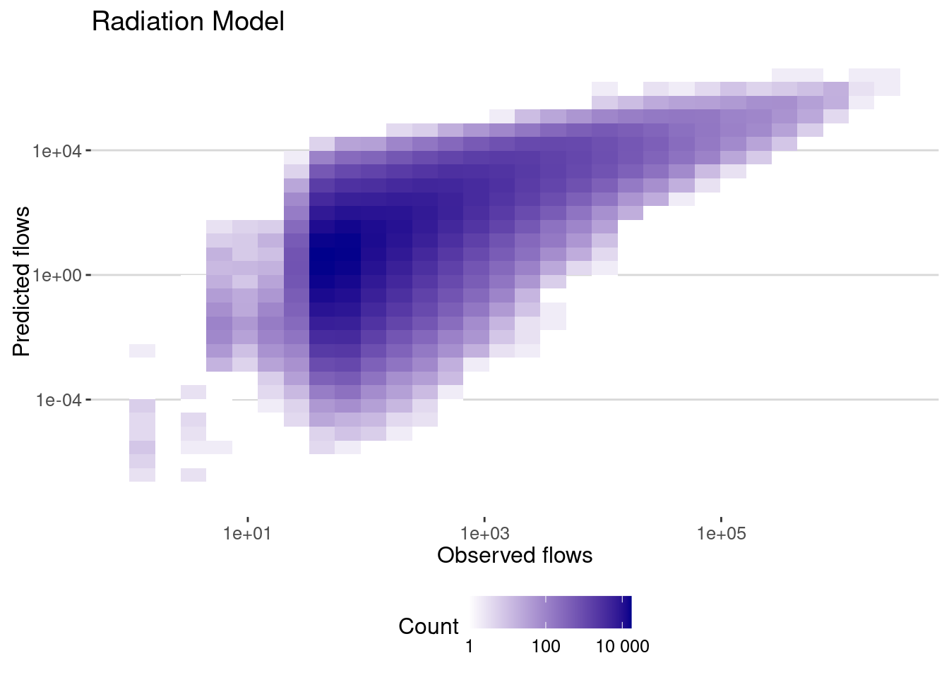
And here is the error of the model:
cor_radiation <- flows_radiation |>
  filter(dist>0) |>
  summarize(cor_values = cor(pop_flows,pred),
            cor_log_values=cor(log(pop_flows),log(pred)),
            cpc = cpc(pop_flows,pred))
cor_radiation
# A tibble: 1 × 3
cor_values cor_log_values cpc
<dbl> <dbl> <dbl>
1 0.692 0.580 0.507As we can see the correlation is very high. And without fitting any parameter!
Summary
Let’s summarize all the models we have
table_results <-
  tibble(model = c("NLS Gravity","LM Gravity Log","LM Gravity Log General","GLM Poisson","GLM Poisson Zeros","Radiation"),
         rbind(cor_gravity_nls,
               cor_gravity_lm,
               cor_gravity_lm_general,
               cor_gravity_glm_poisson,
               cor_gravity_glm_poisson_zeros,
               cor_radiation))
table_results |> datatable()
Your turn
The performance of the gravity models depends a lot on the spatial scale. In general, models work worse at smaller scales, because at small scale details about population density, number of POIs and other geographical barriers matter. Repeat the analysis at the Census tract level and compare the results.
The data for census tracts for the year 2019 can be obtained at the github of the GeoDS Lab. It is already in stella in the /data/CUS/COVID19USFlows-WeeklyFlows-Ct2019 folder.
Let’s load the data using the data.table package for the flows in the week of October 7th 2019.
require(data.table)
files <- Sys.glob("/data/CUS/COVID19USFlows-WeeklyFlows-Ct2019/weekly_flows/ct2ct/2019_10_07/*.csv.gz")
flows_2019 <- lapply(files,fread) |> rbindlist() |>
  mutate(geoid_o = str_pad(geoid_o,11,"left","0"),
         geoid_d = str_pad(geoid_d,11,"left","0"))
Let’s get only the ones in the Boston MSA
counties_in_boston <- c("25021","25009","25017","25025","25023","25005","33015","33017")
flows_boston <- flows_2019 |>
  filter(substr(geoid_o,1,5) %in% counties_in_boston) |>
  filter(substr(geoid_d,1,5) %in% counties_in_boston)
Get the census tract populations
tracts <- get_acs(geography = "tract",
                  variables = "B01003_001",year=2020,
                  state=c("MA","NH"),
                  geometry = TRUE,
                  progress = F) |>
  filter(substr(GEOID,1,5) %in% counties_in_boston)
Plot them
flows_boston |> filter(pop_flows > 800) |>
  ggplot() +
  geom_sf(data=tracts,col="grey",fill="white",alpha=0.5,size=0.01) +
  geom_segment(aes(x=lng_o,y=lat_o,xend=lng_d,yend=lat_d,
                   alpha=log(pop_flows)),size=.5,col="darkgreen") +
  theme_void()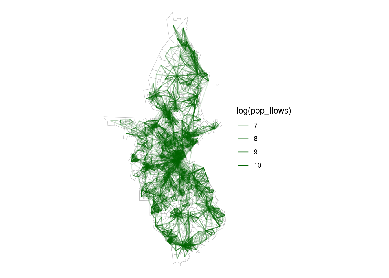
Prepare the data for the model
flows_boston <- flows_boston |>
  mutate(dist = dist_cities_haver(lng_o,lat_o,lng_d,lat_d)) |>
  left_join(tracts |> st_drop_geometry() |> select(GEOID,estimate),
            by=c("geoid_o"="GEOID")) |>
  rename(pop_o = estimate) |>
  left_join(tracts |> st_drop_geometry() |> select(GEOID,estimate),
            by=c("geoid_d"="GEOID")) |>
  rename(pop_d = estimate) |>
  drop_na()
Here is the data. To avoid noise we only select the flows with more than 10 trips and those census areas with more than 10 people.
data_model <- flows_boston |>
  filter(pop_o > 10 & pop_d > 10 & dist > 0 & pop_flows > 50)
Fit that data to different gravity models
NLS
Let’s fit a nls model
gravity_nls <- nls(...)Let’s see the results
data_model |>
  mutate(pred = fitted(gravity_nls)) |>
  ggplot(aes(x=pop_flows,y=pred)) + geom_bin2d() +
  scale_x_log10() + scale_y_log10() +
  scale_fill_continuous(name="Count",
                        trans = "log",
                        low = "white", high = "darkblue",
                        breaks = scales::log_breaks(),  # Set log-based breaks
                        labels = scales::label_number() ) + # Convert labels back to real numbers
  labs(title="NLS Gravity model fit",x="Observed flows",y="Predicted flows")
and the correlation
cor_nls <- data_model |>
  mutate(pred = fitted(gravity_nls)) |>
  summarize(cor_values = cor(pop_flows,pred),
            cor_log_values=cor(log(pop_flows),log(pred)),
            cpc=cpc(pop_flows,pred))
cor_nls
Generalized gravity model
gravity_lm_general <- lm(...)
summary(gravity_model)
cor_gravity_lm_general <- data_model |>
filter(dist>0) |>
mutate(pred = exp(fitted(gravity_model))) |>
summarize(cor_values = cor(pop_flows,pred),
cor_log_values=cor(log(pop_flows),log(pred)),
cpc=cpc(pop_flows,pred))
cor_before_gravity_model_generalRadiation
dist_df <- st_distance(st_centroid(tracts)) |> as.matrix()
colnames(dist_df) <- tracts$GEOID
rownames(dist_df) <- tracts$GEOID
class(dist_df) <- "numeric"
dist_tracts <- dist_df |> as_tibble(rownames="origin") |>
  pivot_longer(cols=-origin,names_to="destination",values_to="distance_m")
Add the population of the destination county
dist_tracts <- dist_tracts |>
  left_join(tracts |> st_drop_geometry() |> select(GEOID,estimate) |>
              rename(pop_dest=estimate),by=c("destination"="GEOID"))
Repeat the steps above to get \(s_{ij}\) and evaluate the radiation model
Conclusions
Population mobility models depend greatly on the spatial scale at which we describe the mobility flows. When choosing which model to use, it is critical to
- Understand the spatial scale of the data, the average distance between units, etc.
- Assuming that the number of flows is proportional to the population and inversely proportional to the distance is a simplification that might not be true.
- We might try other functional forms for the distance, or use travel distance instead of Euclidean distance.
- The radiation model is a good alternative when we do not have a lot of data or when we want to avoid fitting parameters.
References
[1]
Y. Kang, S. Gao, Y. Liang, M. Li, and J. Kruse, “Multiscale dynamic human mobility flow dataset in the u.s. During the COVID-19 epidemic,” Scientific Data, pp. 1–13, 2020.