library(tidyverse)
library(arrow)
options(arrow.unsafe_metadata = TRUE)
library(DT) # for interactive tables
library(knitr) # for tables
library(ggthemes) # for ggplot themes
library(sf) # for spatial data
library(tigris) # for US geospatial data
library(tidycensus) # for US census data
library(fixest) # for fixed effects models
library(stargazer) # for tables
library(leaflet) # for interactive maps
theme_set(theme_hc() + theme(axis.title.y = element_text(angle = 90))) Lab 7 - Causal Inference for Spatial Data
Objective
In this practical, we will use causal inference to understand the effect of interventions or external shocks in urban dynamics. Specifically, we will use mobility data to understand the causal effect of grocery stores on foot traffic on nearby restaurants during COVID-19 shelter-in-place policies. For that purpose we will:
- Explore the data to understand how to define treatment and control groups.
- Use DID methods to estimate the causal effect of the intervention.
- Use synthetic control methods to build conterfactuals.
- Discuss the limitations of the methods and the data.
Load some libraries and settings we will use
Introduction
During COVID-19 lockdowns, city residents restricted their visits only to essential places, like some type of works, groceries, etc. As a result the visit to restaurants, entertainment, transportation declined significantly. Since mobility was highly reduced, restaurants closer to groceries may have benefited from being located near these essential places. In this lab, we will use causal inference methods to understand the effect of grocery stores on foot traffic on nearby restaurants during COVID-19 shelter-in-place policies in the Boston metropolitan area. Our methodology follows the one in [1].
Load mobility data
To get foot traffic to business we will use the Monthly Patterns for Boston Metropolitan since 2019 from Advan, which can be found in the /data/CUS/Boston_Monthly_Patterns folder. Note that in Lab 3-1 we only used the ones for the City of Boston.
files <- Sys.glob("/data/CUS/safegraph/Monthly_Patterns/Boston_MSA_*.parquet")
patterns <- open_dataset(files,format = "parquet")
Again, here is the schema of the data.
schema(patterns)Schema
PLACEKEY: string
PARENT_PLACEKEY: string
SAFEGRAPH_BRAND_IDS: string
LOCATION_NAME: string
BRANDS: string
STORE_ID: double
TOP_CATEGORY: string
SUB_CATEGORY: string
NAICS_CODE: int32
LATITUDE: double
LONGITUDE: double
STREET_ADDRESS: string
CITY: string
REGION: string
POSTAL_CODE: string
OPEN_HOURS: string
CATEGORY_TAGS: string
OPENED_ON: timestamp[us, tz=UTC]
CLOSED_ON: timestamp[us, tz=UTC]
TRACKING_CLOSED_SINCE: timestamp[us, tz=UTC]
WEBSITES: string
GEOMETRY_TYPE: string
POLYGON_WKT: string
POLYGON_CLASS: string
ENCLOSED: bool
PHONE_NUMBER: int64
IS_SYNTHETIC: bool
INCLUDES_PARKING_LOT: bool
ISO_COUNTRY_CODE: string
WKT_AREA_SQ_METERS: int32
DATE_RANGE_START: timestamp[us, tz=UTC]
DATE_RANGE_END: timestamp[us, tz=UTC]
RAW_VISIT_COUNTS: int32
RAW_VISITOR_COUNTS: int32
VISITS_BY_DAY: string
POI_CBG: int64
VISITOR_HOME_CBGS: string
VISITOR_HOME_AGGREGATION: string
VISITOR_DAYTIME_CBGS: string
VISITOR_COUNTRY_OF_ORIGIN: string
DISTANCE_FROM_HOME: int32
MEDIAN_DWELL: int32
BUCKETED_DWELL_TIMES: string
RELATED_SAME_DAY_BRAND: string
RELATED_SAME_MONTH_BRAND: string
POPULARITY_BY_HOUR: string
POPULARITY_BY_DAY: string
DEVICE_TYPE: string
NORMALIZED_VISITS_BY_STATE_SCALING: int32
NORMALIZED_VISITS_BY_REGION_NAICS_VISITS: double
NORMALIZED_VISITS_BY_REGION_NAICS_VISITORS: double
NORMALIZED_VISITS_BY_TOTAL_VISITS: double
NORMALIZED_VISITS_BY_TOTAL_VISITORS: double
See $metadata for additional Schema metadataLet’s select the data and some columns only for groceries and restaurants.
variables <- c("PLACEKEY","LOCATION_NAME","LATITUDE","LONGITUDE",
               "REGION","POSTAL_CODE","TOP_CATEGORY","SUB_CATEGORY",
               "DATE_RANGE_START","RAW_VISIT_COUNTS","RAW_VISITOR_COUNTS")
data <- patterns |>
  filter(TOP_CATEGORY %in% c("Restaurants and Other Eating Places","Grocery Stores")) |>
  select(all_of(variables)) |>
  collect() |>
  mutate(category = ifelse(TOP_CATEGORY == "Restaurants and Other Eating Places","Restaurants","Groceries")) |>
  filter(REGION=="MA")
Here is the aggregated number of visits to restaurants and groceries from 2019 to 2021.
data |>
  filter(year(DATE_RANGE_START) %in% 2020) |>
  group_by(DATE_RANGE_START,category) |>
  summarize(visits = sum(RAW_VISIT_COUNTS,na.rm=T)) |>
  group_by(category) |>
  mutate(visits = visits / visits[month(DATE_RANGE_START)==1]) |>
  ggplot(aes(x=as.Date(DATE_RANGE_START), y=visits, col=category)) + geom_line() +
  labs(title="Visits to groceries and restaurants in Boston",
       subtitle = "Normalized to January 2020",
       x="Date",y="Visits")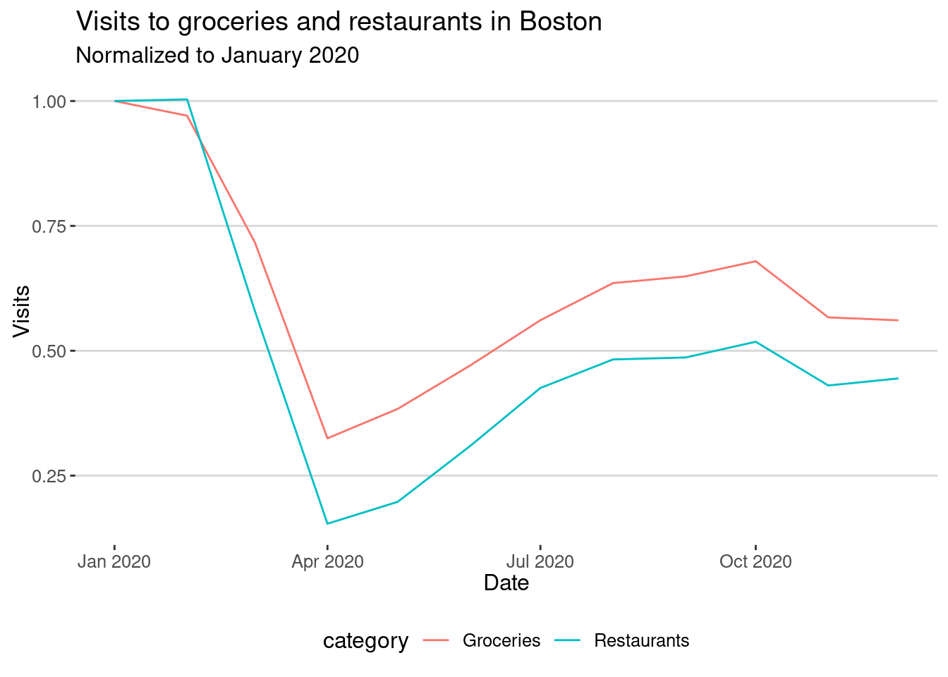
As we can see in the plot, visits to groceries recovered faster than visits to restaurants in the metro area.
Define treatment and control groups
To understand the effect of groceries on restaurants, we need to define treatment and control groups. We will consider the following:
- Treatment group: Restaurants which have a grocery store within \(\delta\) meters of distance.
- Control group: Restaurants which do not have a grocery store within \(\delta\) meters.
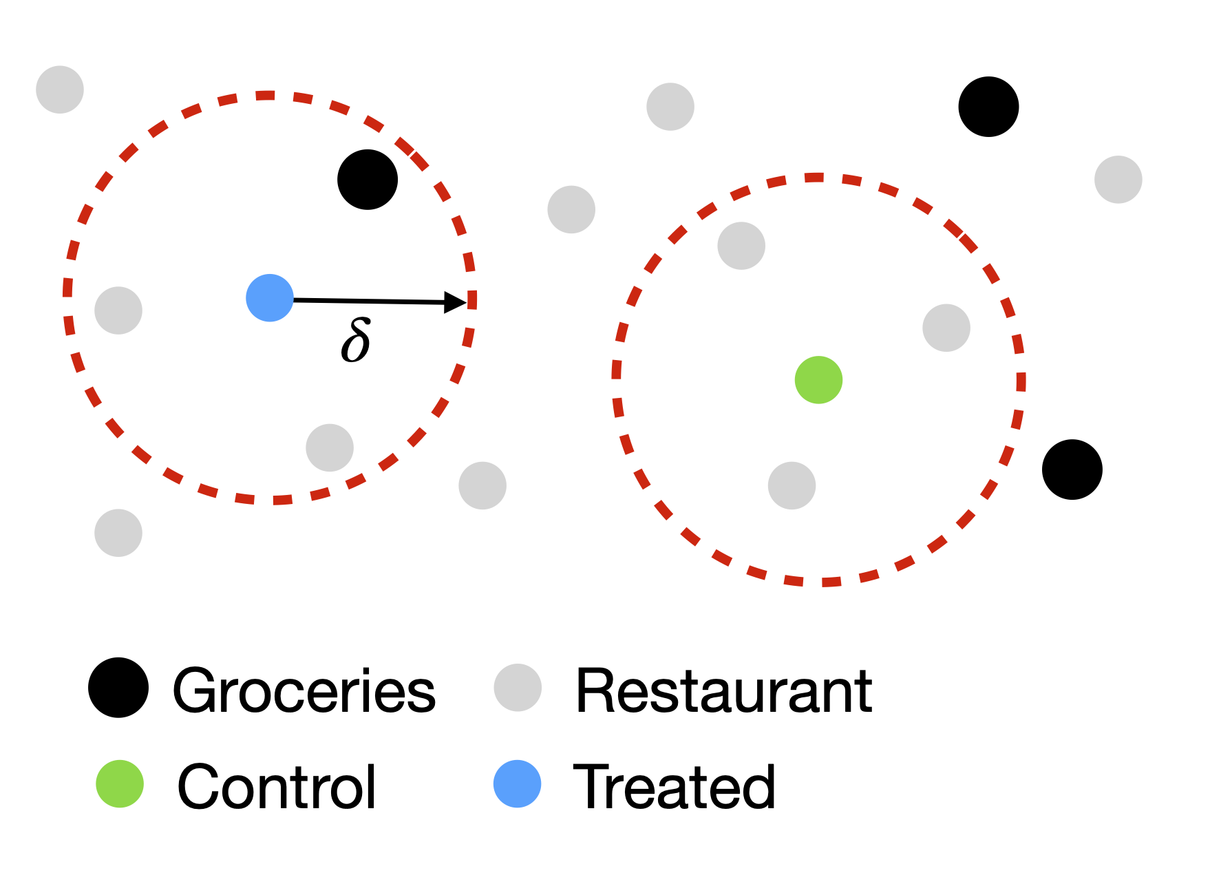
To do this, we will calculate the distance between all restaurants and groceries in the city of Boston.
Caution
Note, be careful, location data for some restaurants changed minimally during the last years, so we will use the first location for each restaurant and grocery.
restaurant_points <- data |>
  filter(category == "Restaurants") |>
  group_by(PLACEKEY) |> slice(1) |>
  st_as_sf(coords = c("LONGITUDE", "LATITUDE"), crs = 4326)
grocery_points <- data |>
  filter(category == "Groceries") |>
  group_by(PLACEKEY) |> slice(1) |>
  st_as_sf(coords = c("LONGITUDE", "LATITUDE"), crs = 4326)
Here is the number of restaurants and groceries
tibble(restaurant = nrow(restaurant_points),grocery = nrow(grocery_points))# A tibble: 1 × 2
restaurant grocery
<int> <int>
1 18161 3340Restaurants and groceries are distributed across the city.
ggplot() +
  geom_sf(data = restaurant_points, col = "grey",alpha=0.5,size=0.5) +
  geom_sf(data = grocery_points, col = "black",alpha=0.5,size=0.5)
Let’s calculate the distance between each restaurant and the closest 5 groceries.
require(nngeo)
distances <- st_nn(restaurant_points,grocery_points,k=5,progress=FALSE)
This is a matrix with the distances between all restaurants and groceries. Let’s find the closest grocery store to each restaurant and get the distance.
dist_closest_grocery <- sapply(distances,min)Now we can calculate the distance to the closest grocery store for each restaurant.
restaurant_points <- restaurant_points |> ungroup() |>
  mutate(dist_closest_grocery = dist_closest_grocery)
Let’s see the distribution of distances to the closest grocery store for restaurants.
restaurant_points |>
  ggplot(aes(x=dist_closest_grocery)) + geom_density() +
  labs(title="Distribution of distances to the closest grocery store for restaurants",
       x="Distance to closest grocery store",y="Density") +
  scale_x_log10()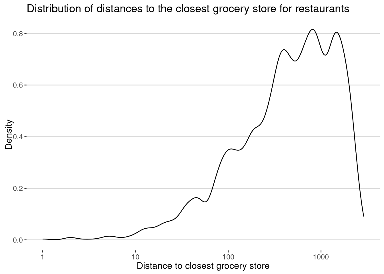
As we can see, the distribution is skewed to the right, with most restaurants having a grocery store nearby (within 1-2km.).
And put that information in the original data.
restaurants <- data |>
  filter(category == "Restaurants") |>
  left_join(restaurant_points %>% select(PLACEKEY,dist_closest_grocery) ,by="PLACEKEY")
Finally, let’s define a control and treatment group based on the distance to the closest grocery store. Given the distribution above, we choose 1000 meters
delta <- 1000
restaurants <- restaurants |>
  mutate(treatment = ifelse(dist_closest_grocery <= delta,1,0))
and see the number of visits to restaurants in the treated and control groups:
restaurants |>
  group_by(treatment,DATE_RANGE_START) |>
  summarize(visits = sum(RAW_VISIT_COUNTS,na.rm=T)) |>
  filter(year(DATE_RANGE_START) %in% 2020) |>
  mutate(visits = visits / sum(visits[month(DATE_RANGE_START) %in% 1:2])) |>
  ggplot(aes(x=as.Date(DATE_RANGE_START),y=visits,col=factor(treatment))) +
  geom_line()+
  labs(title="Normalized number of visits to treated and control restaurants",
       x="Date",y="Visits")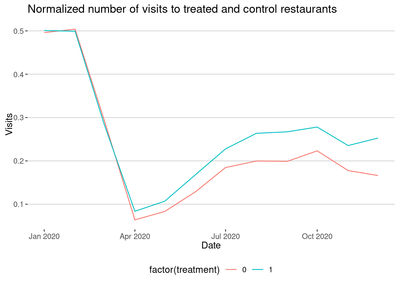
We can already see that the restaurants with a grocery store nearby have more visits than those without a grocery store.
To evaluate better this causal effect we use Difference-in-differences (DID). It compares the change in the outcome variable in the treatment group before and after the intervention with the change in the control group. The difference between these differences is the causal effect of the intervention. In our case, the intervention the lockdown in March 2020.
Let’s calculate the DID estimator for the effect of groceries on restaurants. We will use the following model:
\[ Y_{it} = \alpha + \beta_1 \text{treatment}_i + \beta_2 \text{post}_t + \beta_3 \text{treatment}_i \times \text{post}_t + \epsilon_{it} \]
where \(Y_{it}\) is the number of visits to restaurant \(i\) at time \(t\), \(\text{treatment}_i\) is a dummy variable that equals 1 if \(i\) is a restaurant and has a grocery store within \(\delta\) meters, \(\text{post}_t\) is a dummy variable that equals 1 after the intervention, and \(\epsilon_{it}\) is the error term.
restaurants <- restaurants |>
  mutate(post = ifelse(DATE_RANGE_START >= as.Date("2020-03-15"),1,0))
Let’s estimate the DID model. Note that we don’t include the treatment effect, because we are using PLACEKEY as a fixed effect.
did_1000 <- restaurants |>
  filter(year(DATE_RANGE_START) %in% c(2020)) |>
fixest::feols(log(RAW_VISITOR_COUNTS) ~ post + treatment:post | PLACEKEY)etable(did_1000) did_1000
Dependent Var.: log(RAW_VISITOR_COUNTS)
post -0.7141*** (0.0097)
post x treatment 0.1465*** (0.0118)
Fixed-Effects: -----------------------
PLACEKEY Yes
________________ _______________________
S.E.: Clustered by: PLACEKEY
Observations 131,401
R2 0.88656
Within R2 0.19079
---
Signif. codes: 0 '***' 0.001 '**' 0.01 '*' 0.05 '.' 0.1 ' ' 1As we can see, the coefficient of the interaction term \(\beta_3\) is positive and significant, which means that the presence of a grocery store near a restaurant has a positive effect on the number of visits to the restaurant. The coefficient is around \(\beta_3 \simeq\) 0.1465, which means that restaurants with a grocery store nearby have ATE = \((e^{\beta_3}-1) \times 100\) = 15.78% more visits than those without a grocery store.
Using distance to define the control group
One of the assumptions we made is the control group is defined by restaurants that have no groceries within 1km of distance. However, we cannot be sure that this is the best definition. When working with spatial data, it is always helpful to compare how our results depend on the inner/outer ring definition [1].
deltas <- c(50,100,200,500,750,1000,1500,1750,2000)
ATE_df <- map_dfr(deltas, \(x){
  restaurants <- restaurants |>
    mutate(treatment = ifelse(dist_closest_grocery <= x,1,0))
  did <- restaurants |>
    filter(year(DATE_RANGE_START) %in% 2020) |>
    fixest::feols(log(RAW_VISITOR_COUNTS) ~ post + treatment:post | PLACEKEY)
  return(tibble(delta = x,ATE = (exp(coef(did)["post:treatment"])-1)*100))
})
Here are the results:
ATE_df |>
  ggplot(aes(x=delta,y=ATE)) + geom_line() +
  labs(title="Causal effect of groceries on visits to restaurants by distance",
       x="Distance to closest grocery store",y="ATE (%)")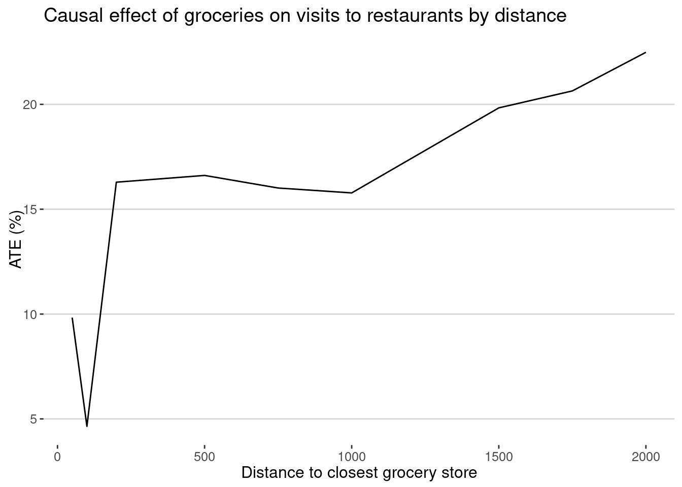
As we can see, the causal effect of groceries on restaurants is positive and significant for all distances, although it is small at small distances. This means that the definition of the control group is crucial to estimating the causal effect of the intervention.
Your turn: continuous treatment
So far, we have assumed that the treatment is binary, i.e., a restaurant either has a grocery store nearby or not. However, we can also consider that treatment is continuous and dependsd on
- The distance to the closest grocery store \(d_{ij}\).
- The number of grocery stores in a radius of \(r\) meters around the restaurant \(i\).
In all these cases, we can estimate the causal effect of groceries on restaurants using a modified DiD model
\[ Y_{it} = \alpha + \beta_1 \text{treat\_intensity}_i + \beta_2 \text{post}_t + \beta_3 \text{treatintensity}_i \times \text{post}_t + \epsilon_{it} \]
Modify the results above to estimate the causal effect of groceries on restaurants using continuous treatment of stores as a continuous variable.
Your turn: CATE
One possibility is that the effect of groceries on restaurants is not the same for all types of restaurants. For example, fast-food restaurants may benefit more from being near a grocery store than fine dining restaurants. To test this hypothesis, estimate the CATE, i.e., the causal effect of groceries on restaurants for different types of restaurants. You can use the SUB_CATEGORY variable to define the types of restaurants.
In the DiD model, you can include the interaction between the treatment and the type of restaurant.
\[ \begin{eqnarray} Y_{it} &=&\alpha + \beta_1 \text{treatment}_i + \beta_2 \text{post}_t + \beta_3 \text{treatment}_i \times \text{post}_t + \\ & & + \beta_4 \text{type}_i + \beta_5 \text{treatment}_i \times \text{post}_t \times \text{type}_i + \epsilon_{it} \end{eqnarray} \] If \(\beta_5\) is positive and significant, it means that the effect of groceries on restaurants is different for different types of restaurants.
Modify the results above to estimate the CATE of groceries on restaurants for different types of restaurants.
Your turn: Confounding Variables
Finally, another possibility is that the causal effect is counfounded by the type of restaurant. For example, the type of restaurants can affect both being exposed to a grocery (fast-food restaurants are more likely to be nearby) and the number of visits after the lockdown (fast-food restaurants were more likely to recover).
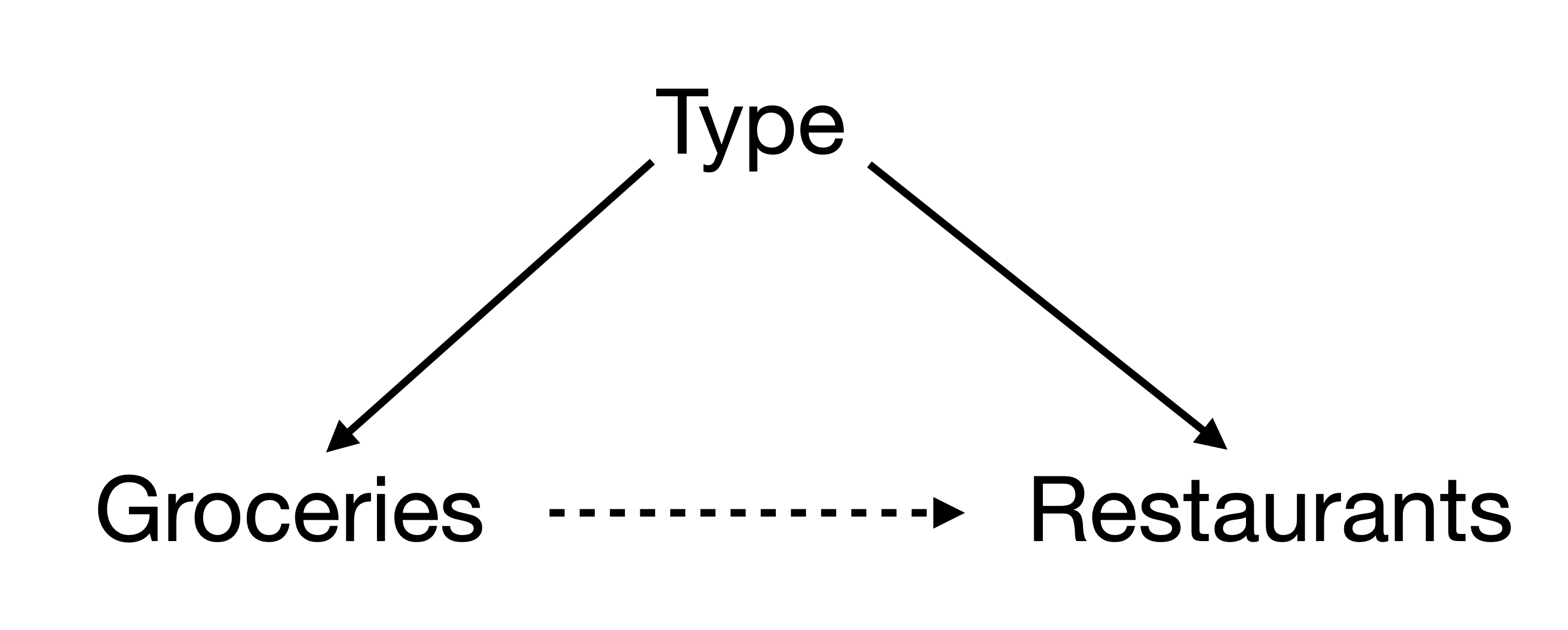
Note that this is different from CATE, where the assumption is that To test this hypothesis, estimate the causal effect of groceries on restaurants using the type of restaurant as a mediator. You can use the following model:
\[ Y_{it} = \alpha + \beta_1 \text{treatment}_i + \beta_2 \text{post}_t + \beta_3 \text{treatment}_i \times \text{post}_t + \beta_4 \text{type}_i + \epsilon_{it} \]
Synthetic control methods (SCM)
Another way to estimate the causal effect of an intervention is to use synthetic control methods [2]. This method constructs a synthetic control group that mimics the treatment group before the intervention. The idea is to find a weighted combination of control units that best approximates the treatment unit before the intervention. In our case, this method can be done for each of the restaurants treated. But for simplicity, let’s put all the visits to the restaurants in the treated group together and use each of the restaurants in the control as donors for the SCM. We will extend it also to the year 2019.
restaurants_SCM <- restaurants |> drop_na(RAW_VISITOR_COUNTS) |>
  filter(year(DATE_RANGE_START) %in% 2019:2020)
We keep only restaurants that appear 24 months in those two years
restaurants_24 <- restaurants_SCM |>
  filter(year(DATE_RANGE_START) %in% 2019:2020) |>
  group_by(PLACEKEY) |>
  summarize(nmonths = sum(!is.na(RAW_VISITOR_COUNTS))) |>
  filter(nmonths == 24) |> select(PLACEKEY) |> pull()
restaurants_SCM <- restaurants_SCM |> filter(PLACEKEY %in% restaurants_24)
We define the treatment and control groups
delta <- 1000
restaurants_SCM <- restaurants_SCM |>
  mutate(treatment = ifelse(dist_closest_grocery <= delta,1,0))
treated_restaurants <- restaurants_SCM |> filter(treatment == 1) |> select(PLACEKEY) |> distinct() |> pull()
control_units <- restaurants_SCM |> filter(treatment == 0) |> select(PLACEKEY) |> distinct() |> pull()
Let’s put together the time series for all of them.
data_treated <- restaurants_SCM |>
  filter(PLACEKEY %in% treated_restaurants) |>
  group_by(DATE_RANGE_START) |>
  summarize(visits = mean(RAW_VISITOR_COUNTS,na.rm=T)) |>
  mutate(index=1) |>
  mutate(month=(year(DATE_RANGE_START)-2019)*12+month(DATE_RANGE_START)) |>
  select(index,month,visits)
For the donors in the control group, let’s use only 100 of them and chose those that have data for all months in the same period. We choose only restaurants that appear 24 months
set.seed(123)
sample_control <- sample(control_units,100)
data_control <- restaurants_SCM |>
  filter(PLACEKEY %in% sample_control) |>
  mutate(index=match(PLACEKEY,sample_control)+1,
         month=(year(DATE_RANGE_START)-2019)*12+month(DATE_RANGE_START),
         visits=RAW_VISITOR_COUNTS)|>
  select(index,month,visits)
The data treated in just one unit
dim(data_treated)[1] 24 3While the control data is for 100 units
dim(data_control)[1] 2400 3In SCM we have to find a combination of the donors that best approximates the treated unit (\(i=1\)) before the intervention.
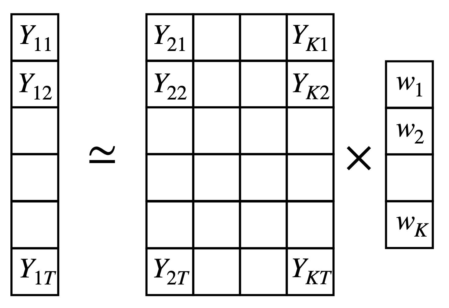
\[ Y_{1t} \simeq \sum_{j \in \text{Donors}} w_j Y_{jt} \] As we know, we have to find the \(w_j\) that minimizes the difference between the treated unit and the synthetic control group before the intervention. We can do this by minimizing the following objective function:
\[ \text{min}_{\sum w_j=1, w_j\geq0} \sum_{t=1}^{T} \left( Y_{1t} - \sum_{j \in \text{Donors}} w_j Y_{jt} \right)^2 \] subject to \(\sum_{j \in \text{Donors}} w_j = 1\) and \(w_j \geq 0\). Not that this equation can be written as matrix equation. If \(X\) is the matrix of the control units (\(X_{tj} = Y_{jt}\)) and \(y\) is the vector of values the treated unit (\(y_t = Y_{1t}\)), we can write the equation as:
\[ min_{||w|| = 0, w_\geq 0 } ||y - Xw||^2 \] where \(w\) is the vector of weights that we want to find.
Let’s build the matrices and the vectors
T <- 15
y <- data_treated |> filter(month < T) |> arrange(month) |> select(visits) |>
  as.matrix()
X <- data_control |> filter(month < T) |> arrange(index,month) |>
  pivot_wider(names_from = index,values_from = visits) |>
  select(-month) |> as.matrix()
Choose an initial guess for the weights
w <- rep(1/ncol(X),ncol(X))Define the loss function
loss_w <- function(w,y,X){
  return(mean((y - X %*% w)^2))
}
And optimize. Note that we don’t normalize weights to one. That can be done always, but it will by just rescaling the output variable.
require(optimx)
get_w <- function(X, y) {
  # Initial weights: Equal distribution
  w_start <- rep(1/ncol(X), ncol(X))

  # Lower and upper bounds (0 <= w_i <= 1)
  lower_bounds <- rep(0, length(w_start))
  upper_bounds <- rep(1, length(w_start))

  # Define a wrapper function to pass X and y correctly
  loss_wrapper <- function(w) loss_w(w, y, X)

  # Perform optimization using optimx
  result <- optimx(
    par = w_start,
    fn = loss_wrapper,
    method = "L-BFGS-B",  # Supports box constraints
    lower = lower_bounds,
    upper = upper_bounds,
    control = list(trace = 0)  # Set to 1 for debugging
  )

  weights <- as.numeric(result[1:length(w_start)])
#  weights <- weights / sum(weights)  # Ensure they sum to 1

  return(weights)
}
Let’s see the weights:
w <- get_w(X,y)
w
[1] 0.014839873 0.000000000 0.048973224 0.011397681 0.011287832 0.011655446
[7] 0.003430901 0.011517029 0.009837776 0.014483408 0.016054871 0.000000000
[13] 0.001593961 0.013812740 0.009749573 0.012976966 0.002772323 0.012515079
[19] 0.011616337 0.010706196 0.021340714 0.002976203 0.009908245 0.003790712
[25] 0.000000000 0.011846482 0.010976826 0.012039398 0.012305742 0.009999971
[31] 0.022960872 0.019079177 0.009789302 0.011903277 0.014070547 0.013476348
[37] 0.009772291 0.011322306 0.020223209 0.014704090 0.011626350 0.011405858
[43] 0.012499942 0.013643120 0.012203187 0.012037772 0.071355075 0.016073759
[49] 0.011152348 0.015587115 0.012652580 0.014752289 0.012170193 0.012435481
[55] 0.011681270 0.003041623 0.008567016 0.010249335 0.013391573 0.018394537
[61] 0.013777859 0.010781192 0.010758611 0.014905945 0.011336841 0.007425106
[67] 0.012973092 0.010415353 0.013819545 0.016181397 0.031331175 0.008101742
[73] 0.000000000 0.002065289 0.011793937 0.033218272 0.053412832 0.011202999
[79] 0.003826622 0.000000000 0.015398274 0.013697322 0.015071923 0.012313407
[85] 0.010430843 0.000000000 0.012408949 0.011239195 0.015014910 0.010391846
[91] 0.012636033 0.012464310 0.009645884 0.012675731 0.028084117 0.008931918
[97] 0.020999061 0.027761564 0.008806043 0.015626460Note that some of the weights are zero, which means that some of the donors are not relevant to construct the synthetic control group.
Let’s see the synthetic control group and the treated unit
y1t <- data_treated |> arrange(month) |> select(visits) |>
  as.matrix()
Xt <- data_control |> arrange(index,month) |>
  pivot_wider(names_from = index,values_from = visits) |>
  select(-month) |> as.matrix()
y0t <- Xt %*% w
dd <- rbind(tibble(month=1:24,type="SCM",visits=y0t[,1]),
            tibble(month=1:24,type="Treated",visits=y1t[,1]))
dd |>
ggplot(aes(x=month,y=visits,col=type)) + geom_line() +
labs(title="Synthetic control group and treated unit",
x="Month Since 2019-01",y="Visits")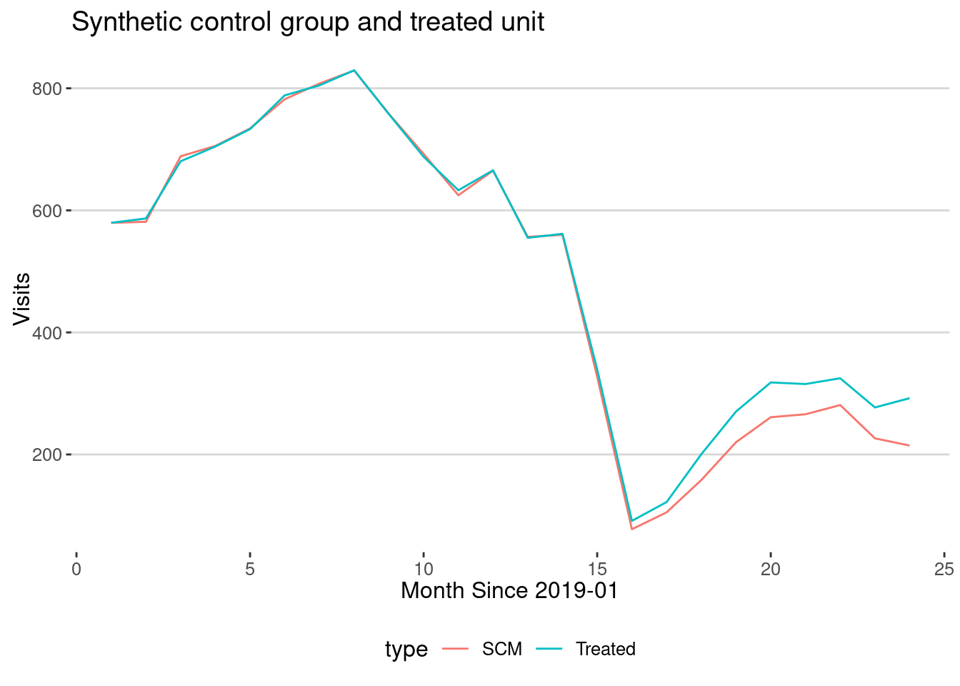
As we can see again, we get that the treated group gets more visits than the synthetic control group. This means that the presence of a grocery store near a restaurant has a positive effect on the number of visits to the restaurant. To be more quantitative, let’s do an DiD on both datasets
data_did_scm <- dd |>
  mutate(post = ifelse(month >= T,1,0)) |>
  mutate(treatment = ifelse(type == "Treated",1,0)) |>
  filter(month >= 12)
fit <- lm(log(visits) ~ post + treatment + treatment:post,data_did_scm)
summary(fit)
Call:
lm(formula = log(visits) ~ post + treatment + treatment:post,
    data = data_did_scm)

Residuals:
     Min       1Q   Median       3Q      Max
-0.95158 -0.06371  0.11698  0.28739  0.50729

Coefficients:
                 Estimate Std. Error t value Pr(>|t|)
(Intercept)     6.3831008  0.2401843  26.576  < 2e-16 ***
post           -1.0999183  0.2738522  -4.016 0.000579 ***
treatment       0.0003434  0.3396719   0.001 0.999202
post:treatment  0.1810794  0.3872855   0.468 0.644697
---
Signif. codes:  0 '***' 0.001 '**' 0.01 '*' 0.05 '.' 0.1 ' ' 1

Residual standard error: 0.416 on 22 degrees of freedom
Multiple R-squared:  0.5611,    Adjusted R-squared:  0.5012
F-statistic: 9.374 on 3 and 22 DF,  p-value: 0.0003483
In this case, we see that although there is a difference between them, our DiD regression is underpowered (only 24 points) to detect it.
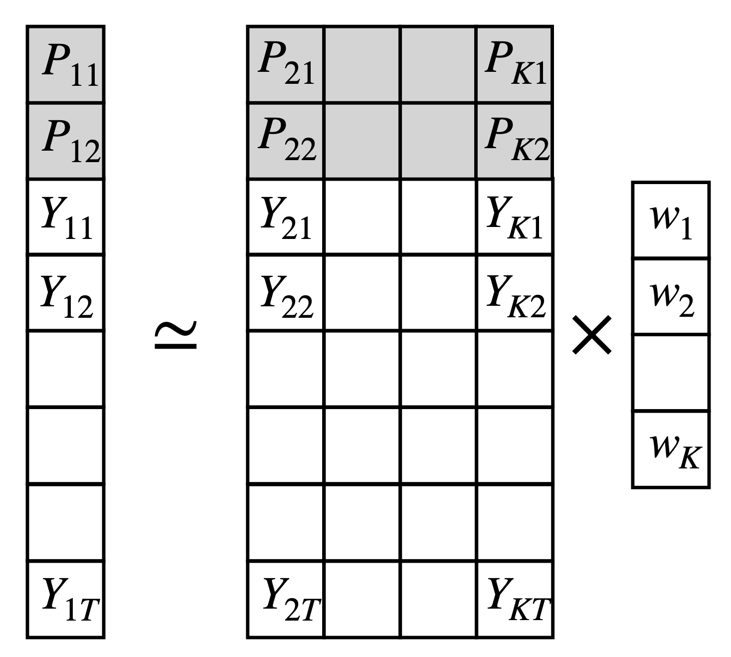
Your turn: SCM with predictors
Finally, we can include predictors in the SCM, i.e. variables we believe are important to construct the synthetic control unit. This mimics the idea of matching in the selection of control units.
To do this, we can plug together the predictors \(P\) to the \(Y_{jt}\) variables and construct a modified \(\hat X = [P | X]\) and a modified \(\hat y = (p, y)\) To do this, we can include these variables in the matrix \(X\) and optimize the weights for them and repeat the analysis above.
 Use the
 POSTAL_CODE and SUB_CATEGORY as predictors and repeat the analysis above.
Conclusions
In this practical exercise, we have used causal inference methods to understand the effect of groceries on restaurants during COVID-19 lockdowns. We have used Difference-in-differences (DID) and synthetic control methods (SCM) to estimate the causal effect of groceries on restaurants.
We have found that the presence of a grocery store near a restaurant has a positive effect on the number of visits to the restaurant. However, the definition of the control group is crucial to estimating the causal effect of the intervention. Thus, always be careful when defining the control group.
References
[1]
M. Pollmann, “Causal Inference for Spatial Treatments.” arXiv, Jan. 2023. doi: 10.48550/arXiv.2011.00373.
[2]
A. Abadie, A. Diamond, and J. Hainmueller, “Synthetic control methods for comparative case studies: Estimating the effect of california’s tobacco control program,” Journal of the American Statistical Association, vol. 105, no. 490, pp. 493–505, 2010, doi: 10.1093/pan/mpr025.