library(tidyverse)
library(arrow) # for efficient dataframes
library(DT) # for interactive tables
library(knitr) # for tables
library(ggthemes) # for ggplot themes
library(sf) # for spatial data
library(tigris) # for US geospatial data
library(tidycensus) # for US census data
library(stargazer) # for tables
library(leaflet) # for interactive maps
library(jsonlite) # for JSON
options(tigris_use_cache = TRUE) # use cache for tigris
theme_set(theme_hc() + theme(axis.title.y = element_text(angle = 90))) Lab 12-2 - Location Intelligence
Objectives
In this lab we will see how to use location data and models to gain insights and make better decisions in the context of grocery stores. To this end
- We will use the Advan data to analyze the number of visitors to each supermarket and the origin of the visitors.
- We will use the Huff model to estimate the probability of a visitor from each census tract visiting each supermarket.
- We will use this model to estimate the effect of closing a supermarket in the City of Boston.
Introduction
Location intelligence is the process of deriving meaningful insights from geospatial data relationships to solve a particular problem. It is a critical component of business intelligence and data analytics.
Location intelligence analyzes spatial data, understands patterns, and makes informed decisions. It is used in various industries, such as retail, real estate, logistics, and marketing.
In this lab, we will use location intelligence to analyze the number of visitors to each grocery store in the Boston MSA and the origin of the visitors. We will use the Huff model to mimic the decision-making of every client to visit a particular supermarket.
Using that model, we can investigate different interventions, such as closing a supermarket, promotional campaigns, the effect of new competitors, etc.
Load some libraries and settings we will use
Load the data
To analyze the visits to different grocery stores, we will use the Monthly Patterns for the Boston Metropolitan Statistical Area (MSA) from the Advan dataset, as we did in Lab 7.
files <- Sys.glob("/data/CUS/safegraph/Monthly_Patterns/Boston_MSA_*.parquet")
patterns <- open_dataset(files,format = "parquet")
Aagin, here is the schema of the data:
patterns |> schema()Schema
PLACEKEY: string
PARENT_PLACEKEY: string
SAFEGRAPH_BRAND_IDS: string
LOCATION_NAME: string
BRANDS: string
STORE_ID: double
TOP_CATEGORY: string
SUB_CATEGORY: string
NAICS_CODE: int32
LATITUDE: double
LONGITUDE: double
STREET_ADDRESS: string
CITY: string
REGION: string
POSTAL_CODE: string
OPEN_HOURS: string
CATEGORY_TAGS: string
OPENED_ON: timestamp[us, tz=UTC]
CLOSED_ON: timestamp[us, tz=UTC]
TRACKING_CLOSED_SINCE: timestamp[us, tz=UTC]
WEBSITES: string
GEOMETRY_TYPE: string
POLYGON_WKT: string
POLYGON_CLASS: string
ENCLOSED: bool
PHONE_NUMBER: int64
IS_SYNTHETIC: bool
INCLUDES_PARKING_LOT: bool
ISO_COUNTRY_CODE: string
WKT_AREA_SQ_METERS: int32
DATE_RANGE_START: timestamp[us, tz=UTC]
DATE_RANGE_END: timestamp[us, tz=UTC]
RAW_VISIT_COUNTS: int32
RAW_VISITOR_COUNTS: int32
VISITS_BY_DAY: string
POI_CBG: int64
VISITOR_HOME_CBGS: string
VISITOR_HOME_AGGREGATION: string
VISITOR_DAYTIME_CBGS: string
VISITOR_COUNTRY_OF_ORIGIN: string
DISTANCE_FROM_HOME: int32
MEDIAN_DWELL: int32
BUCKETED_DWELL_TIMES: string
RELATED_SAME_DAY_BRAND: string
RELATED_SAME_MONTH_BRAND: string
POPULARITY_BY_HOUR: string
POPULARITY_BY_DAY: string
DEVICE_TYPE: string
NORMALIZED_VISITS_BY_STATE_SCALING: int32
NORMALIZED_VISITS_BY_REGION_NAICS_VISITS: double
NORMALIZED_VISITS_BY_REGION_NAICS_VISITORS: double
NORMALIZED_VISITS_BY_TOTAL_VISITS: double
NORMALIZED_VISITS_BY_TOTAL_VISITORS: double
See $metadata for additional Schema metadataWe only need the grocery stores and only some of those variables:
variables <- c("PLACEKEY", "LOCATION_NAME","LATITUDE", "LONGITUDE",
               "REGION","POSTAL_CODE", "TOP_CATEGORY", "SUB_CATEGORY",
               "DATE_RANGE_START", "RAW_VISIT_COUNTS", "RAW_VISITOR_COUNTS",
               "VISITOR_HOME_AGGREGATION")
groceries <- patterns |>
  filter(TOP_CATEGORY == "Grocery Stores") |>
  filter(REGION == "MA") |>
  select(all_of(variables)) |> collect()
Let’s restrict ourselves to only the year 2019
groceries <- groceries |>
  filter(DATE_RANGE_START >= "2019-01-01" & DATE_RANGE_START < "2020-01-01")
Select the major supermarkets
We calculate the total number of visitors to each location
groceries |>
  group_by(PLACEKEY,LOCATION_NAME,SUB_CATEGORY) |>
  summarize(total_visitors = sum(RAW_VISITOR_COUNTS)) |>
  arrange(desc(total_visitors)) |>
  head(10)
# A tibble: 10 × 4
# Groups: PLACEKEY, LOCATION_NAME [10]
PLACEKEY LOCATION_NAME SUB_CATEGORY total_visitors
<chr> <chr> <chr> <int>
1 zzy-22q@62j-qp7-tsq Lean & Green Gourmet Supermarket… 1348358
2 224-224@62j-shy-yvz Caribbean Market Supermarket… 197108
3 226-224@62j-shz-4n5 Boston Phone Card Wholesale … Supermarket… 197108
4 225-227@62j-shz-4n5 Grocery Manufacturers of Ame… Supermarket… 191062
5 zzy-228@62j-shz-4n5 Grillo's Pickles Supermarket… 191062
6 zzy-229@62j-shz-3h5 Sandy's Variety Store Supermarket… 191062
7 zzy-22m@62j-shz-52k Costa's Fruit Stand Supermarket… 191062
8 zzw-233@62k-p76-d7q Alltown Convenience… 182041
9 zzw-223@62j-srj-fj9 Wegmans Food Markets Supermarket… 164995
10 zzy-22s@62j-srj-ffz Sweet Bite Supermarket… 164995As we can see, there are a lot of small places that are also considered as grocery stores. In particular, the first one is a small grocery store in Logan Airport. Let’s keep only the major supermarket brands in the area and that have more than 10 visitors
grocery_brands <- c("Star Market", "Whole Foods Market", "Market Basket",
                    "Stop & Shop", "Wegmans", "Trader Joe's",
                    "Roche Brothers Supermarket")
groceries_table <- groceries |>
  filter(LOCATION_NAME %in% grocery_brands) |>
  group_by(PLACEKEY,LOCATION_NAME) |>
  summarize(total_visitors = sum(RAW_VISITOR_COUNTS,na.rm=T),
            LONGITUDE = mean(LONGITUDE),
            LATITUDE = mean(LATITUDE)) |>
  filter(total_visitors > 10)
Here is the map with each supermarket with different colors and sizes according to the number of visitors
pal <- colorFactor(palette = "Set1", domain = groceries_table$LOCATION_NAME)
leaflet(groceries_table) |>
  addProviderTiles(provider=providers$CartoDB.Positron) |>
  addCircleMarkers(radius = ~sqrt(total_visitors)/10,
                   color = ~ pal(LOCATION_NAME),
                   fillOpacity = 0.8,
                   popup = ~paste0(PLACEKEY,"<br>",
                                   LOCATION_NAME, "<br>",
                                   total_visitors)) |>
  addLegend("bottomright",
            pal=pal,
            values=~LOCATION_NAME,
            title = "Supermarkets")
Analyze the visits to grocery stores
Next, we analyze where visitors to particular grocery stores come from and how they come to them. To do that, we use the VISITOR_HOME_AGGREGATION variable that contains the number of visitors from each census tract that visited the store.
Let’s first get the tracts in the Boston MSA:
variables <- c(
  population = "B01003_001",              # Total Population
  median_household_income = "B19013_001", # Median Household Income
  poverty_rate = "B17001_002"             # Population Below Poverty Level
)
ma_tracts <- get_acs(
  geography = "tract",
  variables = variables,
  state = "MA",
  year = 2022,         # Latest available year
  geometry = TRUE,     # Include spatial data
  output = "wide",
  progress = FALSE
) |>
  st_transform(4326)
ma_tracts <- ma_tracts %>%
  mutate(
    poverty_rate_percent = (poverty_rateE / populationE) * 100
  )
Now, we expand the visits to the store from each census tract as we did in Lab 3-1.
groceries_expanded <- groceries |>
  filter(LOCATION_NAME %in% grocery_brands) |>
  group_by(PLACEKEY,LOCATION_NAME) |>
  mutate(VISITOR_HOME_AGGREGATION = str_replace_all(VISITOR_HOME_AGGREGATION, '""', '"')) |>
  mutate(
    # Parse JSON safely with error handling
    VISITOR_HOME_AGGREGATION =
      map(VISITOR_HOME_AGGREGATION,
          ~ tryCatch(fromJSON(.x),
                     error = function(e) NULL  # Replace errors with NULL
          ))
  ) |>
  filter(!map_lgl(VISITOR_HOME_AGGREGATION, is.null)) |>
  # Expand JSON into rows
  unnest_longer(VISITOR_HOME_AGGREGATION) %>%
  # Rename columns
  rename(Home_ID = VISITOR_HOME_AGGREGATION_id, Count = VISITOR_HOME_AGGREGATION)
As we can see, we now contain one row by grocery store and Home_ID where visitors come from:
groceries_expanded |>
  select(PLACEKEY,LOCATION_NAME,Home_ID,Count) |> head(10)
# A tibble: 10 × 4
# Groups: PLACEKEY, LOCATION_NAME [1]
PLACEKEY LOCATION_NAME Home_ID Count
<chr> <chr> <chr> <int>
1 22h-22v@62k-pd6-wx5 Market Basket 25023503101 98
2 22h-22v@62k-pd6-wx5 Market Basket 25023503102 76
3 22h-22v@62k-pd6-wx5 Market Basket 25023508101 73
4 22h-22v@62k-pd6-wx5 Market Basket 25023504101 53
5 22h-22v@62k-pd6-wx5 Market Basket 25023504102 46
6 22h-22v@62k-pd6-wx5 Market Basket 25023502101 45
7 22h-22v@62k-pd6-wx5 Market Basket 25023505200 43
8 22h-22v@62k-pd6-wx5 Market Basket 25023502200 41
9 22h-22v@62k-pd6-wx5 Market Basket 25023506101 41
10 22h-22v@62k-pd6-wx5 Market Basket 25023506102 37To get more data, let’s aggregate all 2019 visits to each supermarket by census tract during the year
groceries_total <- groceries_expanded |>
  group_by(PLACEKEY, LOCATION_NAME, Home_ID) |>
  summarize(visitors = sum(Count),
            LATITUDE = mean(LATITUDE,na.rm=T),
            LONGITUDE = mean(LONGITUDE,na.rm=T)) |>
  ungroup()
We restrict the visits only to census tracts in the Boston MSA
groceries_total <- groceries_total |>
  filter(Home_ID %in% ma_tracts$GEOID)
For example, this is where users come to visit the Star Market in Prudential (only those with more than 50 visitors)
visitors_start_market <- groceries_total |>
  filter(PLACEKEY == "222-222@62j-sj3-mp9") |>
  left_join(ma_tracts, by = c("Home_ID" = "GEOID")) |>
  filter(visitors > 50)
pal <- colorQuantile("Blues", domain = visitors_start_market$visitors)
visitors_start_market |>
  st_as_sf() |>
  leaflet() |>
  addProviderTiles(provider=providers$CartoDB.Positron) |>
  addPolygons(fillColor = ~pal(visitors),
              fillOpacity = 0.8,
              color = "white",
              weight = 1,
              popup = ~paste0(Home_ID, "<br>",
                              visitors, "<br>")) |>
  addLegend("bottomright",
            pal = pal,
            values = ~visitors,
            title = "Visitors")
For future reference, let’s add the centroid coordinates of each census tract and the distance in our table
ma_tracts_table <- ma_tracts |>
  st_centroid() |>
  st_coordinates() |>
  as.data.frame() |>
  setNames(c("LONGITUDE", "LATITUDE")) |>
  mutate(GEOID = ma_tracts$GEOID,
         pop = ma_tracts$populationE,
         med_income = ma_tracts$median_household_incomeE,
         poverty_rate = ma_tracts$poverty_rate_percent)
Let’s add that and the distance
dist_cities_haver <- function(lon1,lat1,lon2,lat2){
  #calculates distances between points in km
  long1 <- lon1*pi/180; lat1 <- lat1*pi/180
  long2 <- lon2*pi/180; lat2 <- lat2*pi/180
  R <- 6371 # Earth mean radius [km]
  delta.long <- (long2 - long1); delta.lat <- (lat2 - lat1)
  a <- sin(delta.lat/2)^2 + cos(lat1) * cos(lat2) * sin(delta.long/2)^2
  c <- 2 * asin(ifelse(sqrt(a)<1,sqrt(a),1))
  R * c
}

groceries_total <- groceries_total |>
  left_join(ma_tracts_table, by = c("Home_ID" = "GEOID")) |>
  mutate(distance = dist_cities_haver(LONGITUDE.x, LATITUDE.x, LONGITUDE.y, LATITUDE.y))
Let’s add also the total number of visitors to be use as the attractiveness of the supermarket
groceries_total <- groceries_total |>
  left_join(groceries_table |> select(PLACEKEY,total_visitors), by = "PLACEKEY")
Here is the final table
groceries_total |>
  select(PLACEKEY,LOCATION_NAME,Home_ID,visitors,total_visitors,distance,pop) |> head(10)
# A tibble: 10 × 7
PLACEKEY LOCATION_NAME Home_ID visitors total_visitors distance pop
<chr> <chr> <chr> <int> <int> <dbl> <dbl>
1 222-222@62j-prg… Market Basket 250056… 8 11600 86.2 5540
2 222-222@62j-prg… Market Basket 250072… 4 11600 159. 5159
3 222-222@62j-prg… Market Basket 250092… 4 11600 27.8 5095
4 222-222@62j-prg… Market Basket 250092… 4 11600 30.8 6680
5 222-222@62j-prg… Market Basket 250092… 20 11600 31.8 6010
6 222-222@62j-prg… Market Basket 250092… 8 11600 35.1 2570
7 222-222@62j-prg… Market Basket 250092… 4 11600 34.8 5683
8 222-222@62j-prg… Market Basket 250092… 8 11600 27.2 7105
9 222-222@62j-prg… Market Basket 250092… 4 11600 28.8 7102
10 222-222@62j-prg… Market Basket 250092… 4 11600 29.3 4744Model the number of visitors to each supermarket
To model the decision-making process of people going to a particular grocery store, we will use the Huff model. The simplest (constrained) version of the Huff model is that the probability of a visitor from a census tract \(i\) to visit supermarket \(j\) is given by
\[ P_{ij} = \frac{A_j / (d_0 + d_{ij})^\gamma}{\sum_{k} A_k/(d_0 + d_{ik})^\gamma} \] where \(P_{ij}\) is the probability of a visitor from the census tract \(i\) to visit supermarket \(j\), \(A_i\) is the attractiveness of supermarket \(j\) and \(d_{ij}\) is the distance traveled from \(i\) to \(j\) and \(d_0\) is a distance cut-off.
In principle, in the Huff model, both \(A_j\), \(\gamma\), and \(d_0\) can be fitted using real data. However, for simplicity, let’s assume that the attractiveness is given by the total number of people visiting the place in 2019. We also assume that \(d_{ij}\) is the distance between the centroid of the census tract and the supermarket.
Thus, our only free parameters to fit are \(\gamma\) and \(d_0\). Let’s define an error function we want to minimize. We will use the sum of the squared errors between the predicted and real number of visitors. If \(T_{ij}\) is the number of visits fromthe census tract \(i\) to supermarket \(j\) and \(T_{i} = \sum_{j} T_{ij}\), then the error for the Huff model is
\[ Error(\gamma,d_0) = \sum_{i,j} (T_{ij} - T_i P_{ij}[\gamma,d_0])^2 \]
here is the function to calculate the error
error_huff <- function(params){
  data_model <- groceries_total |>
    group_by(Home_ID) |>
    mutate(huff = total_visitors/(params[1]+distance)^params[2]) |>
    mutate(huff = huff/sum(huff)) |>
    mutate(huff_pred = sum(visitors) * huff)
  sum((data_model$visitors - data_model$huff_pred)^2)
}
Finally, we fit \(\gamma\) to minimize the error:
fit <- optim(par = c(1,1),
             fn = error_huff,
             method = "L-BFGS-B",
             lower = c(0,0),
             upper = c(10,10)
)
params_opt <- fit$par
params_opt
[1] 2.732225 2.834513As we can see, the exponent \(\gamma\) is large. This is expected since there are a lot of grocery stores in the area, and thus, distance is very important in deciding where to go.
Let’s plot the number of visitors to each supermarket and the predicted number of visitors.
predictions <- groceries_total |>
  group_by(Home_ID) |>
  mutate(huff = total_visitors/(params_opt[1]+distance)^params_opt[2]) |>
  mutate(huff = huff/sum(huff)) |>
  mutate(huff_pred = sum(visitors) * huff)
predictions |> filter(visitors > 10) |>
ggplot(aes(x=visitors,y=huff_pred)) +
geom_point(alpha=0.1) + scale_x_log10() +
scale_y_log10() +
geom_abline(intercept = 0, slope = 1, color = "darkred",
linetype = "dashed",lwd=1)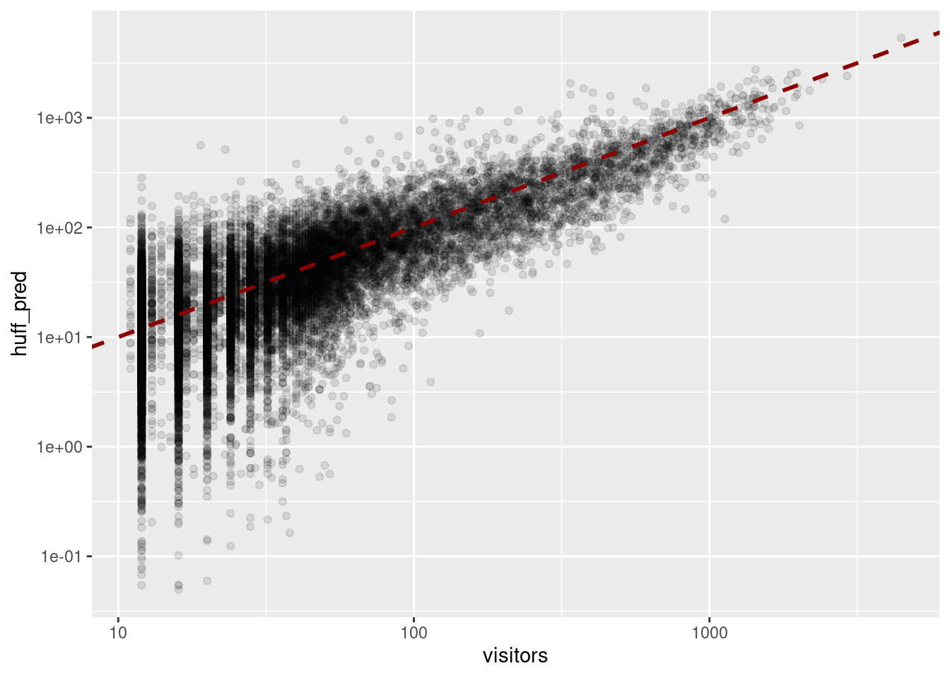
As we can see the model is very good. Let’s quantify that error in terms of the \(R^2\) coefficient
R2 <- cor(predictions$visitors,predictions$huff_pred)^2
R2
[1] 0.7905344Your turn
In this model, we only considered the attractiveness of the place and the distance as possible factors in deciding where to go. Even though the model is very good, what other factors could be considered to improve it?
Effect of closing a supermarket
Suppose that the Star Market in Prudential closes down. How would the number of visitors to each supermarket change? Let’s calculate that using our model:
groceries_no_start_market <- groceries_total |>
  filter(! PLACEKEY == "222-222@62j-sj3-mp9")
predictions_new <- groceries_no_start_market |>
  group_by(Home_ID) |>
  mutate(huff = total_visitors/(params_opt[1] + distance)^params_opt[2]) |>
  mutate(huff = huff/sum(huff)) |>
  mutate(huff_pred = sum(visitors) * huff)
This is the number of visitors before and after
groceries_total_before <- predictions |>
  group_by(PLACEKEY,LOCATION_NAME) |>
  summarize(visitors_before = sum(huff_pred),
            LONGITUDE = mean(LONGITUDE.x),
            LATITUDE = mean(LATITUDE.x))
groceries_total_after <- predictions_new |>
  group_by(PLACEKEY,LOCATION_NAME) |>
  summarize(visitors_after = sum(huff_pred))
groceries_comparison <- groceries_total_before |>
  left_join(groceries_total_after, by = c("PLACEKEY","LOCATION_NAME")) |>
  mutate(visitors_diff = (visitors_after - visitors_before)/visitors_before*100)
The grocery stores that will get more increase in the number of visitors are
groceries_comparison |>
  arrange(desc(visitors_diff)) |>
  select(PLACEKEY,LOCATION_NAME,visitors_diff) |> head(10)
# A tibble: 10 × 3
# Groups: PLACEKEY [10]
PLACEKEY LOCATION_NAME visitors_diff
<chr> <chr> <dbl>
1 226-222@62j-sj3-nyv Trader Joe's 14.8
2 23z-222@62j-sj4-5xq Whole Foods Market 14.1
3 225-222@62j-sgh-9xq Stop & Shop 12.6
4 222-223@62j-sjp-brk Stop & Shop 12.4
5 24p-223@62j-sgj-3qz Star Market 12.1
6 22j-222@62j-sgh-dsq Stop & Shop 12.0
7 22c-222@62j-sjk-6ff Stop & Shop 12.0
8 228-222@62j-sgb-3kf Whole Foods Market 10.6
9 zzw-222@62j-sjg-3bk Stop & Shop 10.5
10 223-222@62j-sjd-6tv Star Market 9.68Here is the map of of the percentage of increase in the number of visitors for all grocery stores
pal <- colorQuantile("RdYlBu", domain = groceries_comparison$visitors_diff)
leaflet(groceries_comparison) |>
  addProviderTiles(provider=providers$CartoDB.Positron) |>
  addCircleMarkers(radius = ~sqrt(abs(visitors_diff))/10,
                   color = ~ pal(visitors_diff),
                   fillOpacity = 0.8,
                   popup = ~paste0(PLACEKEY,"<br>",
                                   LOCATION_NAME, "<br>",
                                   visitors_diff)) |>
  addLegend("bottomright",
            pal=pal,
            values=~visitors_diff,
            title = "Change in visitors")
As expected, the grocery stores near the Star Market in Prudential (Trader Joe’s and Whole Foods) will get more visitors.
Your turn
Suppose the Star Market in Prudential has a promotion, and the number of visitors increases by 10%.
- How would you estimate the increase in visitors from each census tract?
- How would other supermarkets be affected?
Your turn
The model can also be used to optimize the location of a new supermarket. Suppose you are a consultant and have to decide where to open a new supermarket in the Boston MSA.
- How would you estimate the number of visitors to the new supermarket?
- How would you use the model to decide where to open the new supermarket?
- What other factors would you consider?
Conclusions
In this lab, we have seen how to use location data and models to gain insights and make better decisions in the context of grocery stores. We have used the Advan data to analyze the number of visitors to each supermarket and the origin of the visitors.
We have used the Huff model to estimate the probability of a visitor from each census tract visiting each supermarket and use it to estimate changes and interventions in the grocery stores.
Although the model is already very good, it can be improved by considering other factors that could affect people’s decision-making process going to a particular grocery store, like accessibility, prices, etc.
Further reading
Calibrating the dynamic Huff model for business analysis using location big data, by Lian et al., [1]
Location Intelligence for dummies by Carto
The Big Book of Mobile Location Data Use Cases by Quadrant
References
[1]
Y. Liang, S. Gao, Y. Cai, N. Z. Foutz, and L. Wu, “Calibrating the dynamic Huff model for business analysis using location big data,” Transactions in GIS, vol. 24, no. 3, pp. 681–703, 2020, doi: 10.1111/tgis.12624.