library(tidyverse)
library(arrow) # for efficient dataframes
library(DT) # for interactive tables
library(knitr) # for tables
library(ggthemes) # for ggplot themes
library(sf) # for spatial data
library(tigris) # for US geospatial data
library(tidycensus) # for US census data
library(stargazer) # for tables
library(leaflet) # for interactive maps
library(jsonlite) # for JSON
options(tigris_use_cache = TRUE) # use cache for tigris
theme_set(theme_hc() + theme(axis.title.y = element_text(angle = 90))) Lab 13-2 - Experienced segregation
Objectives
In this practical, we will analyze the experienced segregation of visitors to social infrastructure places in the Boston MSA. To do that,t we will:
- Use large-scale data from the Advan dataset to study the income diversity of visitors to different places.
- Compute the experienced segregation of visitors to different places.
- Analyze the geographical distribution of segregation in the Boston MSA.
- Analyze the segregation by category of place.
Introduction
Segregation is a complex phenomenon that can be studied from different perspectives. In this practical, we will analyze the experienced segregation of visitors to social infrastructure places in the Boston MSA.
Most studies of segregation rely on residential information. However, the segregation of visitors to places can be very different from that of residents. For example, a place can be visited by people from different income groups, even if the place is located in a high-income neighborhood.
Thus, there is a vast difference between residential segregation (how similar people live in the same area) and experienced segregation (how similar people visit the same place). Several research works have found that experienced segregation is mainly determined by the category of the places visited and the lifestyle of people, not where they live [1], [2], [3]. This challenges the impact of residential segregation on experienced segregation.

In this practical, we will analyze the experienced segregation of visitors to social infrastructure places in the Boston MSA [4]. We will use the Advan dataset to study the income diversity of visitors to different places. We will compute the experienced segregation of visitors to different places and analyze the geographical distribution of segregation in the Boston MSA. We will also explore the segregation by category of place.
Load some libraries and settings we will use
Load the data
To analyze the visits to different places, we will use the Monthly Patterns for the Boston Metropolitan Statistical Area (MSA) from the Advan dataset, as we did in Lab 7 and Lab 12-2
files <- Sys.glob("/data/CUS/safegraph/Monthly_Patterns/Boston_MSA_*.parquet")
patterns <- open_dataset(files,format = "parquet")
Again, here is the schema of the data:
patterns |> schema()Schema
PLACEKEY: string
PARENT_PLACEKEY: string
SAFEGRAPH_BRAND_IDS: string
LOCATION_NAME: string
BRANDS: string
STORE_ID: double
TOP_CATEGORY: string
SUB_CATEGORY: string
NAICS_CODE: int32
LATITUDE: double
LONGITUDE: double
STREET_ADDRESS: string
CITY: string
REGION: string
POSTAL_CODE: string
OPEN_HOURS: string
CATEGORY_TAGS: string
OPENED_ON: timestamp[us, tz=UTC]
CLOSED_ON: timestamp[us, tz=UTC]
TRACKING_CLOSED_SINCE: timestamp[us, tz=UTC]
WEBSITES: string
GEOMETRY_TYPE: string
POLYGON_WKT: string
POLYGON_CLASS: string
ENCLOSED: bool
PHONE_NUMBER: int64
IS_SYNTHETIC: bool
INCLUDES_PARKING_LOT: bool
ISO_COUNTRY_CODE: string
WKT_AREA_SQ_METERS: int32
DATE_RANGE_START: timestamp[us, tz=UTC]
DATE_RANGE_END: timestamp[us, tz=UTC]
RAW_VISIT_COUNTS: int32
RAW_VISITOR_COUNTS: int32
VISITS_BY_DAY: string
POI_CBG: int64
VISITOR_HOME_CBGS: string
VISITOR_HOME_AGGREGATION: string
VISITOR_DAYTIME_CBGS: string
VISITOR_COUNTRY_OF_ORIGIN: string
DISTANCE_FROM_HOME: int32
MEDIAN_DWELL: int32
BUCKETED_DWELL_TIMES: string
RELATED_SAME_DAY_BRAND: string
RELATED_SAME_MONTH_BRAND: string
POPULARITY_BY_HOUR: string
POPULARITY_BY_DAY: string
DEVICE_TYPE: string
NORMALIZED_VISITS_BY_STATE_SCALING: int32
NORMALIZED_VISITS_BY_REGION_NAICS_VISITS: double
NORMALIZED_VISITS_BY_REGION_NAICS_VISITORS: double
NORMALIZED_VISITS_BY_TOTAL_VISITS: double
NORMALIZED_VISITS_BY_TOTAL_VISITORS: double
See $metadata for additional Schema metadatasocial_infraestructure <- c("Museums, Historical Sites, and Similar Institutions",
"Religious Organizations","Other Schools and Instruction",
"Elementary and Secondary Schools",
"Business Schools and Computer and Management Training",
"Junior Colleges","Social Assistance",
"Civic and Social Organizations","Performing Arts Companies",
"Social Advocacy Organizations",
"Individual and Family Services",
"Technical and Trade Schools",
"Colleges, Universities, and Professional Schools")Let’s get only those type of places and only some of those variables:
variables <- c("PLACEKEY", "LOCATION_NAME","LATITUDE", "LONGITUDE",
               "REGION","POSTAL_CODE", "TOP_CATEGORY", "SUB_CATEGORY",
               "DATE_RANGE_START", "RAW_VISIT_COUNTS", "RAW_VISITOR_COUNTS",
               "VISITOR_HOME_AGGREGATION")
social <- patterns |>
  filter(TOP_CATEGORY %in% social_infraestructure) |>
  filter(REGION == "MA") |>
  select(all_of(variables)) |> collect()
For simplicity, we only consider the year 2019:
social <- social |>
  filter(DATE_RANGE_START >= "2019-01-01" & DATE_RANGE_START < "2020-01-01")
Data exploration
We calculate the total number of visitors to each location:
social |>
  group_by(PLACEKEY,LOCATION_NAME,SUB_CATEGORY) |>
  summarize(total_visitors = sum(RAW_VISITOR_COUNTS)) |>
  arrange(desc(total_visitors)) |>
  head(20) |> datatable()
As we can see, there are a lot of small places that have a large number of visitors. This is because they belong to the same place (Esplanade area in Boston). We can filter them out later.
Analyze the demographics of the visitors
To analyze the visitors’ demographics, we need to determine where they are coming from. To do that, we use the VISITOR_HOME_AGGREGATION variable that contains the number of visitors from each census tract that visited the store.
Let’s first get the tracts in the Boston MSA:
variables <- c(
  population = "B01003_001",              # Total Population
  median_household_income = "B19013_001", # Median Household Income
  poverty_rate = "B17001_002"             # Population Below Poverty Level
)
ma_tracts <- get_acs(
  geography = "tract",
  variables = variables,
  state = "MA",
  year = 2022,         # Latest available year
  geometry = TRUE,     # Include spatial data
  output = "wide",
  progress = FALSE
) |>
  st_transform(4326)
ma_tracts <- ma_tracts %>%
  mutate(
    poverty_rate_percent = (poverty_rateE / populationE) * 100
  )
To study the income profile of visits, let’s add a quantile by income to the table:
ma_tracts <- ma_tracts |>
  mutate(income_quantile = ntile(median_household_incomeE, 4))
Now, we expand the visits to the store from each census tract as we did in Lab 3-1.
social_expanded <- social |>
  group_by(PLACEKEY,LOCATION_NAME) |>
  mutate(VISITOR_HOME_AGGREGATION = str_replace_all(VISITOR_HOME_AGGREGATION, '""', '"')) |>
  mutate(
    # Parse JSON safely with error handling
    VISITOR_HOME_AGGREGATION =
      map(VISITOR_HOME_AGGREGATION,
          ~ tryCatch(fromJSON(.x),
                     error = function(e) NULL  # Replace errors with NULL
          ))
  ) |>
  filter(!map_lgl(VISITOR_HOME_AGGREGATION, is.null)) |>
  # Expand JSON into rows
  unnest_longer(VISITOR_HOME_AGGREGATION) %>%
  # Rename columns
  rename(Home_ID = VISITOR_HOME_AGGREGATION_id, Count = VISITOR_HOME_AGGREGATION)
As we can see, we now contain one row by place and Home_ID where visitors come from:
social_expanded |>
  select(PLACEKEY,LOCATION_NAME,Home_ID,Count) |> head(10)
# A tibble: 10 × 4
# Groups: PLACEKEY, LOCATION_NAME [1]
PLACEKEY LOCATION_NAME Home_ID Count
<chr> <chr> <chr> <int>
1 zzw-223@62k-nz5-fs5 Oak Street Elementary 25021442103 59
2 zzw-223@62k-nz5-fs5 Oak Street Elementary 25021442101 45
3 zzw-223@62k-nz5-fs5 Oak Street Elementary 25021442102 37
4 zzw-223@62k-nz5-fs5 Oak Street Elementary 25021442202 22
5 zzw-223@62k-nz5-fs5 Oak Street Elementary 25021442201 12
6 zzw-223@62k-nz5-fs5 Oak Street Elementary 25027755200 8
7 zzw-223@62k-nz5-fs5 Oak Street Elementary 25021441204 6
8 zzw-223@62k-nz5-fs5 Oak Street Elementary 25005630200 4
9 zzw-223@62k-nz5-fs5 Oak Street Elementary 25005630300 4
10 zzw-223@62k-nz5-fs5 Oak Street Elementary 25021410100 4To get more data, let’s aggregate all 2019 visits to each place by census tract during the year
social_total <- social_expanded |>
  group_by(PLACEKEY, LOCATION_NAME, Home_ID) |>
  summarize(visitors = sum(Count),
            LATITUDE = mean(LATITUDE,na.rm=T),
            LONGITUDE = mean(LONGITUDE,na.rm=T)) |>
  ungroup()
We restrict the visits only to census tracts in the Boston MSA
social_total <- social_total |>
  filter(Home_ID %in% ma_tracts$GEOID)
Calculating experienced segregation by POI
To calculate the experienced segregation by POI, we need to measure the diversity of visitors to a place. In this practical we concentrate on income diversity. Thus, we add the quantile of income for visitors coming from different tracts.
social_total <- social_total |>
  left_join(ma_tracts |> select(GEOID,income_quantile) |> st_drop_geometry(),
            by = c("Home_ID" = "GEOID")) |>
  filter(!is.na(income_quantile))
There are different ways of measuring segregation. Here, we will use an extension of the Dissimilarity Index to more than 2 groups, as suggested in [1]. The formula is:
\[ S_\alpha = \frac{2}{3} \sum_{q=1}^4 |\tau_{\alpha q} - \frac14| \] where \(\tau_{\alpha q}\) is the proportion of group \(q\) in place \(\alpha\). If only one group visits the place, the index is \(S_\alpha = 1\). If the place is visited equally by all groups, then \(S_\alpha = 0\).
Let’s calculate the experienced segregation for each place
social_segregation <- social_total |>
  group_by(PLACEKEY,LOCATION_NAME) |>
  summarize(
    S = 2/3 * sum(abs(table(income_quantile) / n() - 1/4)),
    n_visitors = sum(visitors),
    n_tracts = n_distinct(Home_ID),
    LATITUDE = mean(LATITUDE),
    LONGITUDE = mean(LONGITUDE)
  ) |>
  arrange(desc(S))
Here is the distribution of place segregation:
social_segregation |> filter(n_visitors > 1000) |>
  ggplot(aes(S)) +
  geom_histogram(bins = 30, fill = "skyblue", color = "black") +
  labs(title = "Distribution of experienced segregation by place",
       x = "Segregation index", y = "Number of places") +
  theme_minimal()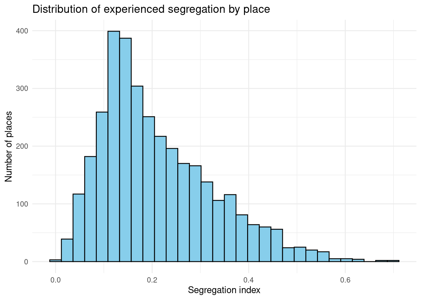
Mapping the segregation
Let’s map the segregation of the places in the Boston MSA
vis_social_segregation <- social_segregation |> filter(n_visitors > 1000)
palette_quantile <- colorQuantile(
  palette = c("blue","green","gold","red"),
  domain = vis_social_segregation$S,
  n = 4  # number of quantiles/colors
)
leaflet(vis_social_segregation) |>
  addProviderTiles(provider = providers$CartoDB.DarkMatter) |>
  addCircleMarkers(
    radius = ~log(n_visitors/100),
    color = ~ palette_quantile(S),
    fillOpacity = 0.8,
    stroke = FALSE,
    popup = ~paste0(LOCATION_NAME, " <br>",
                    "Segregation: ", round(S,2), "<br>",
                    "Visitors: ", n_visitors)
  ) |>
  addLegend("bottomright", pal = palette_quantile,
    values = ~S, title = "Segregation",
    opacity = 1
  )
Segregation by Category of place
Let’s add the category of the place to the table with social segregation
social_segregation <- social_segregation |>
  left_join(social |>
              select(PLACEKEY, LOCATION_NAME, TOP_CATEGORY, SUB_CATEGORY) |>
              distinct(), by = c("PLACEKEY", "LOCATION_NAME"))
Here is the distribution of segregation values by category of place as violin plot. We only consider those categories with more than 100 places:
social_segregation |> filter(n_visitors > 50) |>
  group_by(TOP_CATEGORY) |>
  filter(n() > 20) |>
  ggplot(aes(y = S, x = TOP_CATEGORY)) +
  geom_violin(fill = "skyblue",alpha=0.5) +
  geom_boxplot(width = 0.1, fill = "white") +
  labs(title = "Distribution of experienced segregation by category of place",
       x = "Category of place", y = "Segregation index") +
  theme_minimal() +
  theme(axis.text.x = element_text(angle = 45, hjust = 1)) +
  coord_flip()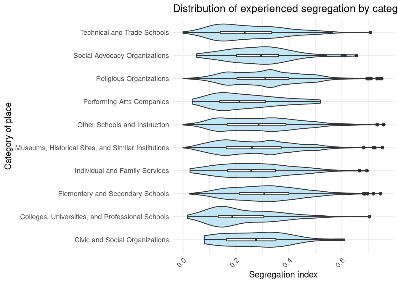
As we can see, on average, Colleges and Art places are less segregated than civic and social organizations, social advocacy organizations, schools, and religious organizations.
Your turn
Redo the analysis of limited-service restaurants in the Boston MSA.
You can use the following code to get the data:
variables <- c("PLACEKEY", "LOCATION_NAME","LATITUDE", "LONGITUDE",
               "REGION","POSTAL_CODE", "TOP_CATEGORY", "SUB_CATEGORY",
               "DATE_RANGE_START", "RAW_VISIT_COUNTS", "RAW_VISITOR_COUNTS",
               "VISITOR_HOME_AGGREGATION")
fastfood <- patterns |>
  filter(SUB_CATEGORY=="Limited-Service Restaurants") |>
  filter(REGION == "MA") |>
  select(all_of(variables)) |> collect()
fastfood_expanded <- fastfood |>
group_by(PLACEKEY,LOCATION_NAME) |>
mutate(VISITOR_HOME_AGGREGATION = str_replace_all(VISITOR_HOME_AGGREGATION, '""', '"')) |>
mutate(
# Parse JSON safely with error handling
VISITOR_HOME_AGGREGATION =
map(VISITOR_HOME_AGGREGATION,
~ tryCatch(fromJSON(.x),
error = function(e) NULL # Replace errors with NULL
))
) |>
filter(!map_lgl(VISITOR_HOME_AGGREGATION, is.null)) |>
# Expand JSON into rows
unnest_longer(VISITOR_HOME_AGGREGATION) %>%
# Rename columns
rename(Home_ID = VISITOR_HOME_AGGREGATION_id, Count = VISITOR_HOME_AGGREGATION) fastfood_total <- fastfood_expanded |>
group_by(PLACEKEY, LOCATION_NAME, Home_ID) |>
summarize(visitors = sum(Count),
LATITUDE = mean(LATITUDE,na.rm=T),
LONGITUDE = mean(LONGITUDE,na.rm=T)) |>
ungroup()We restrict the visits only to census tracts in the Boston MSA
fastfood_total <- fastfood_total |>
  filter(Home_ID %in% ma_tracts$GEOID)
To calculate the experienced segregation by POI, we need to measure the diversity of visitors to a place. First we add their quantile of income
fastfood_total <- fastfood_total |>
  left_join(ma_tracts |> select(GEOID,income_quantile) |> st_drop_geometry(),
            by = c("Home_ID" = "GEOID")) |>
  filter(!is.na(income_quantile))
Let’s calculate the experienced segregation for each place
fastfood_total <- fastfood_total |>
  group_by(PLACEKEY,LOCATION_NAME) |>
  summarize(
    S = 2/3 * sum(abs(table(income_quantile) / n() - 1/4)),
    n_visitors = sum(visitors),
    n_tracts = n_distinct(Home_ID),
    LATITUDE = mean(LATITUDE),
    LONGITUDE = mean(LONGITUDE)
  ) |>
arrange(desc(S))- Find the distribution of segregation in those places.
- Map the segregation of the places in the Boston MSA.
- Calculate the distribution of segregation values by company as violin plot.
- Which are the most segregated fast food places in the Boston area?
Conclusions
We have analyzed the experienced segregation of visitors to social infrastructure places in the Boston MSA.
- Event places in the same category can have very different segregation patterns.
- Geographically, we see that high- and low- segregated places can coexist in the same areas, challenging the idea of segregation as a residential problem.
- We have found that, on average, Colleges and Art places are less segregated than civic and social organizations, social advocacy organizations, schools, and religious organizations.
- This is expected, as some of those civil organizations serve local communities.
Note that, for simplicity, we haven’t post-stratified the data in our calculations. Post-stratification is crucial to minimize the effect of potential biases of the data in our metric. As we know, Advan data is biased by income, so this becomes important in our results. We leave that part for future work.
Further reading
Here are some papers that use similar data and methods to study experienced segregation:
- Mobility patterns are associated with experienced income segregation in large {US} cities [1]
- Estimating experienced racial segregation in US cities using large-scale GPS data [2]
- Using human mobility data to quantify experienced urban inequalities [3]
- The great equalizer? Mixed effects of social infrastructure on diverse encounters in cities, [4],
References
[1]
E. Moro, D. Calacci, X. Dong, and A. Pentland, “Mobility patterns are associated with experienced income segregation in large US cities,” Nature Communications, vol. 12, no. 1, pp. 1–10, Jul. 2021, doi: 10.1038/s41467-021-24899-8.
[2]
S. Athey, B. Ferguson, M. Gentzkow, and T. Schmidt, “Estimating experienced racial segregation in US cities using large-scale GPS data,” Proceedings of the National Academy of Sciences, vol. 118, no. 46, p. e2026160118, Nov. 2021, doi: 10.1073/pnas.2026160118.
[3]
F. Xu et al., “Using human mobility data to quantify experienced urban inequalities,” Nature Human Behaviour, pp. 1–11, Feb. 2025, doi: 10.1038/s41562-024-02079-0.
[4]
T. Fraser, T. Yabe, D. P. Aldrich, and E. Moro, “The great equalizer? Mixed effects of social infrastructure on diverse encounters in cities,” Computers, Environment and Urban Systems, vol. 113, p. 102173, Oct. 2024, doi: 10.1016/j.compenvurbsys.2024.102173.